Personal Savings in the US Following the COVID Relief Programs, and the Possible Impact in 2023 and 2024

A.  Introduction

The US economy has just gone through an extraordinary period.  The impacts are still being felt – and probably will be for several more years, including into the presidential election year of 2024.  A key issue will be whether personal consumption expenditures will continue to grow – at least at some modest pace – as such expenditures are important not only in themselves, but also as they account for more than two-thirds of the demand side of GDP.  And this consumption will depend, in turn, on what happens to household incomes and on the decisions households make on their savings.

Very briefly, we will find:

a)  Personal Income before taxes and transfers (at the national level as measured in the GDP accounts, and where taxes and transfers are for all levels of government including state and local in addition to federal) fell during the Covid crisis but then recovered to where it was before by mid-2021.  Since then, however, it has been relatively flat in real terms.

b)  Personal Income after taxes and transfers (called Disposable Personal Income in the GDP accounts) rose during the Covid crisis due to the massive Covid relief packages, but returned to its previous trend path by mid-2021.  But as the Covid relief programs wound down, Disposable Personal Income (in real terms) fell, and by October 2022 was almost 7% below its previous trend path.

This stagnation in Personal Income, and fall in Disposable Personal Income, may well explain the common view of many that the economy is not well, despite unemployment rates that have matched the lowest levels of more than the last half-century.

c)  But while Disposable Personal Income fell below its trend path, Personal Consumption Expenditure (which had fallen during the Covid crisis) returned fully to its previous trend path by the Spring of 2021.  It has since followed that trend path almost exactly.

d)  This return of Personal Consumption to its previous trend path, while Disposable Personal Income fell well below its previous trend path, was only possible as households could draw on large savings balances that they had built up during the Covid crisis period.

e)  Those savings balances are finite, however, and are being drawn down.  While only a crude estimate is possible, calculations based on the savings rates that prevailed before the Covid crisis and then extrapolation based on the pace of the drawdown in 2022, suggest that the excess savings balances will be depleted sometime in 2024.

This may have significant implications, both economically and politically.  The Fed is currently raising interest rates aggressively in order to reduce investment spending and hence aggregate demand, with the objective of reducing inflation.  Federal fiscal spending has also been falling, with a reduction expected in FY2023 of a further about 1% of GDP.  Many analysts (including myself) have felt that a reduction in consumer expenditures in 2023 (as the excess savings balances built up during the Covid crisis run out) should be expected on top of this.  But based on the calculations discussed below, those balances might last into 2024.  That makes 2024 a complicated year economically, and 2024 is a presidential election year.

The possible macro consequences will be discussed in the concluding section of this post.  They are necessarily more speculative.  But first we will look at what happened to the savings rate during and following the Covid crisis (the chart at the top of this post), and then what happened to Personal Incomes, Disposable Personal Incomes, and Personal Consumption Expenditures – both in terms of their levels and relative to their previous trend paths.  The penultimate section will then provide an estimate of how much excess savings was built up during the Covid crisis period, the pace at which it is now being drawn down, and how long such balances might last before being used up.

A note on usage:  When terms such as personal incomes or personal consumption expenditures are capitalized, they are referring to the specific concepts as measured in the published GDP accounts (or more properly, the National Income and Product Accounts, or NIPA).  Terms that are not capitalized refer to the concepts more generally.  And I made one modification: “Personal Current Transfer Receipts” is defined in the NIPA accounts as net of social insurance (Social Security and Medicare) taxes paid.  I instead include such taxes in the category of Personal Current Taxes (i.e. together with individual income taxes), and Personal Transfers are then just the gross transfers (from Social Security, etc.).

B.  The Personal Savings Rate

The personal savings rate jumped sharply with the onset of the Covid crisis in March 2020.  From a rate of between 6 and 8% of disposable incomes for most of the period between 2013 and 2019, and reaching 9% in 2019 and early 2020, the rate jumped to 14% in March and then 34% in April 2020.  Such a jump is unprecedented in peacetime.  The only time there has been anything similar was during World War II.

The data for this chart (and those below) were calculated from data published by the Bureau of Economic Analysis (BEA) as part of the National Income and Product Accounts.  And while the GDP estimates themselves are only presented on a quarterly basis, the BEA provides monthly estimates for Personal Income, its sources (wages, etc.), Personal Taxes paid and Transfers received, and how the income thus derived is then used for consumption expenditures and other outlays, and residually for Personal Savings.  See in particular Table 2.6 in the NIPA accounts.  All the figures used here are seasonally adjusted and (where relevant) at annual rates.

The Personal Savings rate is defined as Personal Savings as a share of Disposable Personal Income, where Disposable Personal Income is Personal Income as received in the market (from wages; interest, dividends, and rents received; and income from unincorporated businesses) less Personal Taxes paid plus Personal Transfers received.  These Personal Transfers include that received from Social Security, Medicare, Medicaid, Veterans’ benefits, unemployment compensation, and other such programs, but during the Covid crisis there were also major transfers from the various Covid relief bills (the direct stimulus checks, the paycheck protection program, grants to small as well as large businesses, and much more) as well as from a large jump in unemployment compensation.

The series of Covid relief measures were huge.  The total appropriated under the six packages passed for Covid relief (five while Trump was president and one early in the Biden administration) sums to $5.7 trillion.  To put this in perspective, the total paid in federal individual income taxes each year is only about $2.6 trillion.  Spread over two years, the $5.7 trillion came to 12.8% of the GDP of 2020 and 2021 together.  A bit more than two-thirds of that money was appropriated under the bills signed into law by Trump, and a bit less than one-third by Biden.  And while the appropriations were passed by Congress with bipartisan (indeed often unanimous) support while Trump was president, the American Rescue Plan signed by Biden on March 11, 2021, received zero votes from Republicans in Congress.

The Covid relief bills provided massive transfers to households (in addition to massive transfers to the corporate sector as well).  But especially with the lockdowns, and then continuing to a lesser extent once the lockdowns were lifted due to Covid concerns (thus leading to less travel, less eating out at restaurants, etc.), consumption expenditures by households fell.  Much of the transfers received under the Covid relief bills hence ended up accumulating in savings balances (including regular bank accounts).  One can see in the chart at the top of this post the peaks in April 2020, January 2021, and March 2021.  These coincided with when what is commonly referred to as the “stimulus checks” – of $1,200, $600, and $1,400 respectively – were sent out.

As conditions normalized, the savings rate came down as the Covid relief measures wound down and as consumption recovered.  But then the savings rate continued to fall to levels well below those of 2019 and before.  The next section will review what was behind this.

C.  Personal Incomes, Personal Disposable Income, and Consumption

The paths followed for Personal Income and its components, from 2013 through to October 2022, are shown in the following chart:

The top three curves show the levels (in constant 2012 dollars) of Personal Income before Taxes and Transfers (in black), Disposable Personal Income (in purple), and Personal Outlays (in orange).  Personal Outlays are in essence almost the same as Personal Consumption Expenditures, but not quite.  Personal Consumption Expenditures accounted for almost all of Personal Outlays consistently throughout this period (never less than 96.0% nor more than 97.1%), but Personal Outlays also include non-mortgage interest payments (mortgage interest is included in housing expenditures) and small amounts of transfers of households to the rest of the world (i.e. overseas, probably mostly to family) and to government.  But since Personal Outlays are almost entirely Personal Consumption Expenditures, and their paths almost identical (just shifted slightly due to the steady 96 to 97% share), we will use the two concepts interchangeably for the purposes here.

The light blue lines on top of each are the simple linear regression lines of the paths from January 2013 to February 2020 – a period where each of the paths were extraordinarily stable – and with each then extrapolated at that same trend pace through to October 2022.  Not only was there little fluctuation in the paths between January 2013 and February 2020, but it was the same path through both the second term of Obama and the first three years of Trump (followed by the crash in Trump’s fourth year).  Indeed, the paths were so stable that the light blue lines of the linear regressions almost obscure the black, purple, and orange paths of the underlying data – up to February 2020.

This then changed abruptly in March 2020 with the onset of the Covid crisis.  But before getting to that, we should discuss the three additional curves in the lower part of the chart.  Shown are the amounts paid in Personal Current Taxes (in red), Personal Current Transfers (in green), and Personal Savings (in brown).  Personal Savings will equal Disposable Personal Income less Personal Outlays (which, as noted above, are basically Personal Consumption Expenditures).

Starting in March 2020, Personal Savings shot upward.  This was due to a combination of the far higher transfers (in green – under the first of the major Covid relief packages), the lower Personal Outlays (in orange – due to the lockdowns and general caution in going out to spend money due to the spread of the virus that causes Covid), and, to a lesser extent, lower taxes paid (in red – as the Covid relief measures included allowing tax payments to be deferred).  With a good deal of volatility (as a consequence of the timing of the major Covid relief packages), this continued through 2020 and to roughly the spring of 2021.

The resulting impacts on Personal Incomes (before and after taxes and transfers) and on Personal Outlays are shown in the upper right of the chart.  A blow-up of this section of the chart may make this easier to follow:

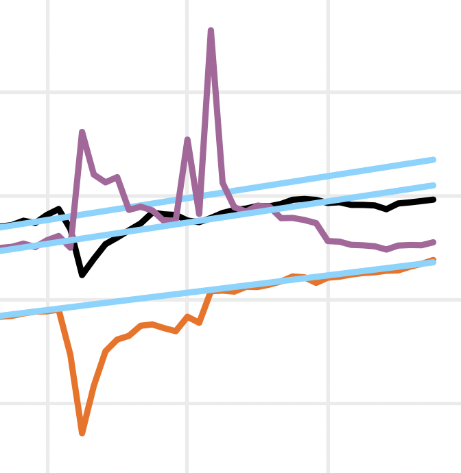
Personal Incomes (before taxes and transfers) recovered quickly, albeit only partially, as the lockdowns were lifted in 2020.  They then continued to rise, although at a slower pace, to the latter part of 2021 as the general economy recovered.  Since then, they have been largely flat.  By October 2022, they were 4.6% below where they would have been had they continued to follow their light-blue regression line for their path prior to March 2020.

Disposable Personal Incomes (i.e. after taxes and transfers) rose during the Covid crisis due to the Covid relief packages – as these more than offset the reduction in Personal Incomes during the crisis (when GDP fell and unemployment rose).  But by mid-2021, Disposable Personal Incomes had come down to the level of Personal Incomes before taxes and transfers, and then continued to fall as the Covid packages wound down.  By October 2022, Disposable Personal Incomes were almost 7% below where they would have been had they continued to follow their light-blue regression line for their path prior to March 2020.

In sharp contrast to Personal Incomes (before or after taxes and transfers), Personal Outlays (or Consumption Expenditures) returned to their previous path by March 2021, and since then have followed that previous path almost exactly.  They could do this only because households could draw down on the high savings balances they had built up during the Covid crisis period.  But there is only so much in those savings balances.  How long might they last?

D.  Excess Savings Balances

Savings rates shot up with the onset of the Covid crisis – due to the transfers received and the difficulties in spending – but the savings balances are now being drawn down.  While the resulting growth in private consumption expenditures has accounted for much of the growth in the demand for GDP in 2021 and continuing into 2022, those excess savings balances cannot last forever.

A crude calculation can be made of how much might be in those savings balances and how long they might last.  It can only be crude as one cannot know with any certainty how much would have been saved in the absence of the Covid crisis and all the impacts it had, nor can one know what returns might have been earned on those savings balances (returns that would depend on how they might have been invested – or not).

Savings rates were relatively stable between 2013 and early 2020 (as seen in the chart at the top of this post), and it is reasonable to assume savings rates would have been similar in the absence of the Covid crisis.  For the purposes here, I looked at scenarios where the savings rate would have remained at its average over 2013 to 2019 (which was 7.3%), or at its somewhat higher average over 2017 to 2019 (of 7.9%).  I also assumed, in part for simplicity, that there was no return earned on these excess savings balances.  This is not unreasonable, as much of what was received under the Covid relief packages were left to accumulate in bank accounts where there was no return.  Interest rates on CDs and such have also been very low for most of this period (and negative when adjusted for inflation).  And to the extent the funds were invested in the stock market (or in bitcoins!), the returns will depend very much on precisely when the investments were made.  The markets were going up for much of the period but now have come down – and sharply.

When the actual savings rates were higher than those assumed in the scenarios (of 7.3% or 7.9%), an excess savings balance was built up, and when the actual savings rates were below these benchmarks, these savings balances were brought down.  Expressed as a share of GDP, the resulting excess balances were:

The balances grew, often rapidly, to March 2021 and then peaked in August 2021 at about 10 to 11% of GDP (depending on what base savings rate is assumed).  Since then, those balances have come down.  Based on the pace of their fall in the most recent six months, they could last for another 18 or 23 months – i.e. for another one and a half to two years – depending on the base savings rate assumed.  That is, they would carry over into 2024, and possibly be all used up just prior to election day in 2024.

There is a good deal of uncertainty in any such forecast – in part due to the factors discussed above that make any such estimate of excess savings balances only approximate.  But there are also issues in what might transpire going forward.  The estimate that the balances might last for another year and a half to two years is based on a simple extrapolation of the extent to which such balances (as imperfectly estimated) have come down over the past half year.  That pace might accelerate.  For example, if Disposable Personal Income widens further from its trend path (this might have stopped in the last few months, but it is still early and hard to say), while Personal Consumption continues to rise according to its trend path, then Personal Savings will fall further and the pace at which the savings balances will be brought down will accelerate.  On the other hand, if the economy weakens and unemployment rises, consumers may become more cautious and decide to conserve their savings balances.

So one should draw only broad conclusions.  But the data does suggest that the excess savings balances built up during the Covid crisis remain significant, and could provide support to continued growth in Personal Consumption Expenditures for some time – perhaps a year or more.  Many had assumed – including me before I looked at the data in this way – that the strong Personal Consumption Expenditures of the last two years would be diminishing soon, as excess savings balances were being used up.  But this data suggests that strong consumption growth might persist for another year or more.  What does this imply for the macro economy?

E.  Macro Implications

Inflation has been high – at 6 to over 8% year-on-year by various measures.  This is far in excess of the goal of the Fed of an inflation rate of around 2%.  In response, the Fed has been aggressively raising the short-term interest rates it controls, as well as reducing its holdings of bonds on its balance sheet (with the aim of raising longer-term interest rates).  Higher interest rates can be expected to reduce demand for investment (in particular in long-lived assets such as housing and other structures), and this lower demand will reduce pressures on prices.

Inflation had averaged around 2% – or even less – since the mid-1990s, but then rose as the economy recovered from the Covid crisis.  As discussed above, Personal Consumption Expenditures recovered quickly and strongly, with this made possible by the high savings balances that had been built up following the series of Covid relief packages while consumption was limited.  But the strong consumption expenditure demands that followed in 2021 and 2022 then faced often limited supplies due to supply chain difficulties as well as the cutbacks in production generally during the peak of the Covid crisis in 2020.  And some items of production cannot be placed into an inventory to be sold later.  For example, a restaurant produces meals for diners, but a meal that was not produced and sold during the Covid crisis cannot simply be kept somewhere and then sold later.  The meal not produced is gone forever.

The result has been a classic “demand-pull” inflation.  While the labor market is now tight, with unemployment the lowest it has been for more than a half-century, increases in nominal wages have fallen short of inflation.  That is, real wages have been falling, and one cannot attribute the inflation observed as primarily stemming from cost-push factors.

The Fed is thus raising interest rates to limit investment demand, and hence aggregate demand.  Whether it will be able to do this without sparking a general recession is the challenge it is facing.  While not impossible, it will certainly be tricky.  In addition, federal fiscal policy will also likely be acting in the direction of reducing demand.  Federal fiscal expenditures fell sharply in FY2022, as the Covid relief packages wound down.  As I write this, Congress has yet to approve a budget for FY2023, but the most recent forecast of the Congressional Budget Office (from July) was that federal fiscal expenditures would fall a further 1.2% of GDP in FY2023.  And with Republicans controlling the House starting in January, it is not likely that fiscal spending will be allowed to respond should the need arise next year due to a downturn developing.

In this sensitive balance of policies – with the Fed seeking to constrain demand but not by too much, and fiscal expenditures unresponsive should conditions change – what will happen to personal consumption expenditures will be critical.  A concern of many has been that such consumption expenditures might also be abruptly reduced once the excess in savings balances built up during the Covid crisis had become used up.  Inflation might well then come down quickly, but possibly with the economy falling into a recession as well.

The analysis above suggests that personal consumption expenditures – growing as it has over the last year and a half – could still be sustained through 2023.  If so, the likelihood of a recession in 2023 will be reduced (although still possible – depending on what the Fed does).  But conditions in 2024 might well then become more difficult to manage.  With the House controlled by the Republicans, who have said they will seek to force through cuts in the federal budget (as they did following their election win in 2010), a fiscal response to the changing conditions might not be forthcoming.  The Fed may be forced to switch rapidly from raising interest rates to cutting them, in an effort to stem a downturn.

It will likely not be easy to manage.  And with 2024 a presidential election year, there may well also be political factors complicating any response.

The Simple Economics of What Determines the Foreign Trade Balance: Econ 101

“There’s no reason that we should have big trade deficits with virtually every country in the world.”

“We’re like the piggybank that everybody is robbing.”

“the United States has been taken advantage of for decades and decades”

“Last year,… [the US] lost  … $817 billion on trade.  That’s ridiculous and it’s unacceptable.”

“Well, if they retaliate, they’re making a mistake.  Because, you see, we have a tremendous trade imbalance. … we can’t lose”

Statements made by President Trump at the press conference held as he left the G-7 meetings in, Québec, Canada, June 9, 2018.


A.  Introduction

President Trump does not understand basic economics.  While that is not a surprise, nor something necessarily required or expected of a president, one should expect that a president would appoint advisors who do understand, and who would tell him when he is wrong.  Unfortunately, this president has been singularly unwilling to do so.  This is dangerous.

Trump is threatening a trade war.  Not only by his words at the G-7 meetings and elsewhere, but also by a number of his actions on trade and tariffs in recent months, Trump has made clear that he believes that a trade deficit is a “loss” to the nation, that countries with trade surpluses are somehow robbing those (such as the US) with a deficit, that raising tariffs can and will lead to reductions in trade deficits, and that if others then also raise their tariffs, the US will in the end necessarily “win” simply because the US has a trade deficit to start.

This is confused on many levels.  But it does raise the questions of what determines a country’s trade balance; whether a country “loses” if it has a trade deficit; and what is the role of tariffs.  This Econ 101 blog post will first look at the simple economics of what determines a nation’s trade deficit (hint:  it is not tariffs); will then discuss what tariffs do and where do they indeed matter; and will then consider the role played by foreign investment (into the US) and whether a trade deficit can be considered a “loss” for the nation (a piggybank being robbed).

B.  What Determines the Overall Trade Deficit?

Let’s start with a very simple case, where government accounts are aggregated together with the rest of the economy.  We will later then separate out government.

The goods and services available in an economy can come either from what is produced domestically (which is GDP, or Gross Domestic Product) or from what is imported.  One can call this the supply of product.  These goods and services can then be used for immediate consumption, or for investment, or for export.  One can call this the demand for product.  And since investment includes any net change in inventories, the goods and services made available will always add up to the goods and services used.  Supply equals demand.

One can put this in a simple equation:

GDP + Imports = Domestic Consumption + Domestic Investment + Exports

Re-arranging:

(GDP – Domestic Consumption) – Domestic Investment = Exports – Imports

The first component on the left is Domestic Savings (what is produced domestically less what is consumed domestically).  And Exports minus Imports is the Trade Balance.  Hence one has:

Domestic Savings – Domestic Investment = Trade Balance

As one can see from the way this was derived, this is simply an identity – it always has to hold.  And what it says is that the Trade Balance will always be equal to the difference between Domestic Savings and Domestic Investment.  If Domestic Savings is less than Domestic Investment, then the Trade Balance (Exports less Imports) will be negative, and there will be a trade deficit.  To reduce the trade deficit, one therefore has to either raise Domestic Savings or reduce Domestic Investment.  It really is as straightforward as that.

Where this becomes more interesting is in determining how the simple identity is brought about.  But here again, this is relatively straightforward in an economy which, like now, is at full employment.  Hence GDP is essentially fixed:  It cannot immediately rise by either employing more labor (as all the workers who want a job have one), nor by each of those laborers suddenly becoming more productive (as productivity changes only gradually through time by means of either better education or by investment in capital).  And GDP is equal to labor employed times the productivity of each of those workers.

In such a situation, with GDP at its full employment level, Domestic Savings can only rise if Domestic Consumption goes down, as Domestic Savings equals GDP minus Domestic Consumption.  But households want to consume, and saving more will mean less for consumption.  There is a tradeoff.

The only other way to reduce the trade deficit would then be to reduce Domestic Investment.  But one generally does not want to reduce investment.  One needs investment in order to become more productive, and it is only through higher productivity that incomes can rise.

Reducing the trade deficit, if desirable (and whether it is desirable will be discussed below), will therefore not be easy.  There will be tradeoffs.  And note that tariffs do not enter directly in anything here.  Raising tariffs can only have an impact on the trade balance if they have a significant impact for some reason on either Domestic Savings or Domestic Investment, and tariffs are not a direct factor in either.  There may be indirect impacts of tariffs, which will be discussed below, but we will see that the indirect effects actually could act in the direction of increasing, not decreasing, the trade deficit.  However, whichever direction they act in, those indirect effects are likely to be small.  Tariffs will not have a significant effect on the trade balance.

But first, it is helpful to expand the simple analysis of the above to include Government as a separate set of accounts.  In the above we simply had the Domestic sector.  We will now divide that into the Domestic Private and the Domestic Public (or Government) sectors.  Note that Government includes government spending and revenues at all levels of government (state and local as well as federal).  But the government deficit is primarily a federal government issue.  State and local government entities are constrained in how much of a deficit they can run over time, and the overall balance they run (whether deficit or surplus) is relatively minor from the perspective of the country as a whole.

It will now also be convenient to write out the equations in symbols rather than words, and we will use:

GDP = Gross Domestic Product

C = Domestic Private Consumption

I = Domestic Private Investment

G = Government Spending (whether for Consumption or for Investment)

X = Exports

M = Imports

T = Taxes net of Transfers

Note that T (Taxes net of Transfers) will be the sum total of all taxes paid by the private sector to government, minus all transfers received by the private sector from government (such as for Social Security or Medicare).  I will refer to this as simply net Taxes (T).

The basic balance of goods or services available (supplied) and goods or services used (demanded) will then be:

GDP + M = C + I + G + X

We will then add and subtract net Taxes (T) on the right-hand side:

GDP + M = (C + T) + I + (G – T) + X

Rearranging:

GDP – (C + T) – (G – T) – I = X – M

(GDP – C – T) – I + (T – G) = X – M

Or in (abbreviated) words:

Dom. Priv. Savings – Dom. Priv. Investment + Govt Budget Balance = Trade Balance

Domestic Private Savings (savings by households and private businesses) is equal to what is produced in the economy (GDP), less what is privately consumed (C), less what is paid in net Taxes (T) by the private sector to the public sector.  Domestic Private Investment is simply I, and includes investment both by private businesses and by households (primarily in homes).  And the Government Budget Balance is equal to what government receives in net Taxes (T), less what Government spends (on either consumption items or on public investment).  Note that government spending on transfers (e.g. Social Security) is already accounted for in net Taxes (T).

This equation is very much like what we had before.  The overall Trade Balance will equal Domestic Private Savings less Domestic Private Investment plus the Government Budget Balance (which will be negative when a deficit, as has normally been the case except for a few years at the end of the Clinton administration).  If desired, one could break down the Government Budget Balance into Public Savings (equal to net Taxes minus government spending on consumption goods and services) less Public Investment (equal to government spending on investment goods and services), to see the parallel with Domestic Private Savings and Domestic Private Investment.  The equation would then read that the Trade Balance will equal Domestic Private Savings less Domestic Private Investment, plus Government Savings less Government Investment.  But there is no need.  The budget deficit, as commonly discussed, includes public spending not only on consumption items but also on investment items.

This is still an identity.  The balance will always hold.  And it says that to reduce the trade deficit (make it less negative) one has to either increase Domestic Private Savings, or reduce Domestic Private Investment, or increase the Government Budget Balance (i.e. reduce the budget deficit).  Raising Domestic Private Savings implies reducing consumption (when the economy is at full employment, as now).  Few want this.  And as discussed above, a reduction in investment is not desirable as investment is needed to increase productivity over time.

This leaves the budget deficit, and most agree that it really does need to be reduced in an economy that is now at full employment.  Unfortunately, Trump and the Republican Congress have moved the budget in the exact opposite direction, primarily due to the huge tax cut passed last December, and to a lesser extent due to increases in certain spending (primarily for the military).  As discussed in an earlier post on this blog, an increase in the budget deficit to a forecast 5% of GDP at a time when the economy is at full employment is unprecedented in peacetime.

What this implies for the trade balance is clear from the basic identity derived above.  An increase in the budget deficit (a reduction in the budget balance) will lead, all else being equal, to an increase in the trade deficit (a reduction in the trade balance).  And it might indeed be worse, as all else is not equal.  The stated objective of slashing corporate taxes is to spur an increase in corporate investment.  But if private investment were indeed to rise (there is in fact little evidence that it has moved beyond previous trends, at least so far), this would further worsen the trade balance (increase the trade deficit).

Would raising tariffs have an impact?  One might argue that this would raise net Taxes paid, as tariffs on imports are a tax, which (if government spending is not then also changed) would reduce the budget deficit.  While true, the extent of the impact would be trivially small.  The federal government collected $35.6 billion in all customs duties and fees (tariffs and more) in FY2017 (see the OMB Historical Tables).  This was less than 0.2% of FY2017 GDP.  Even if all tariffs (and other fees on imports) were doubled, and the level of imports remained unchanged, this would only raise 0.2% of GDP.  But the trade deficit was 2.9% of GDP in FY2017.  It would not make much of a difference, even in such an extreme case.  Furthermore, new tariffs are not being pushed by Trump on all imports, but only a limited share (and a very limited share so far).  Finally, if Trump’s tariffs in fact lead to lower imports of the items being newly taxed, as he hopes, then tariffs collected can fall.  In the extreme, if the imports of such items go to zero, then the tariffs collected will go to zero.

Thus, for several reasons, any impact on government revenues from the new Trump tariffs will be minor.

The notion that raising tariffs would be a way to eliminate the trade deficit is therefore confused.  The trade balance will equal the difference between Domestic Savings and Domestic Investment.  Adding in government, the trade balance will equal the difference between Domestic Private Savings and Domestic Private Investment, plus the equivalent for government (the Government Budget Balance, where a budget deficit will be a negative).  Tariffs have little to no effect on these balances.

C.  What Role Do Tariffs Play, Then?

Do tariffs then matter?  They do, although not in the determination of the overall trade deficit.  Rather, tariffs, which are a tax, will change the price of the particular import relative to the price of other products.  If applied only to imports from some countries and not from others, one can expect to see a shift in imports towards those countries where the tariffs have not been imposed.  And in the case when they are applied globally, on imports of the product from any country, one should expect that prices for similar products made in the US will then also rise.  To the extent there are alternatives, purchases of the now more costly products (whether imported or produced domestically) will be reduced, while purchases of alternatives will increase.  And there will be important distributional changes.  Profits of firms producing the now higher priced products will increase, while the profits of firms using such products as an input will fall.  And the real incomes of households buying any of these products will fall due to the higher prices.

Who wins and who loses can rapidly become turn into something very complicated.  Take, for example, the new 25% tariff being imposed by the Trump administration on steel (and 10% on aluminum).  The tariffs were announced on March 8, to take effect on March 23.  Steel imports from Canada and Mexico were at first exempted, but later the Trump administration said those exemptions were only temporary.  On March 22 they then expanded the list of countries with temporary exemptions to also the EU, Australia, South Korea, Brazil, and Argentina, but only to May 1.  Then, on March 28, they said imports from South Korea would receive a permanent exemption, and Australia, Brazil, and Argentina were granted permanent exemptions on May 2.  After a short extension, tariffs were then imposed on steel imports from Canada, Mexico, and the EU, on May 31.  And while this is how it stands as I write this, no one knows what further changes might be announced tomorrow.

With this uneven application of the tariffs by country, one should expect to see shifts in the imports by country.  What this achieves is not clear.  But there are also further complications.  There are hundreds if not thousands of different types of steel that are imported – both of different categories and of different grades within each category – and a company using steel in their production process in the US will need a specific type and grade of steel.  Many of these are not even available from a US producer of steel.  There is thus a system where US users of steel can apply for a waiver from the tariff.  As of June 19, there have been more than 21,000 petitions for a waiver.  But there were only 30 evaluators in the US Department of Commerce who will be deciding which petitions will be granted, and their training started only in the second week of June.  They will be swamped, and one senior Commerce Department official quoted in the Washington Post noted that “It’s going to be so unbelievably random, and some companies are going to get screwed”.  It would not be surprising to find political considerations (based on the interests of the Trump administration) playing a major role.

So far, we have only looked at the effects of one tariff (with steel as the example).  But multiple tariffs on various goods will interact, with difficult to predict consequences.  Take for example the tariff imposed on the imports of washing machines announced in late January, 2018, at a rate of 20% in the first year and at 50% should imports exceed 1.2 million units in the year.  This afforded US producers of washing machines a certain degree of protection from competition, and they then raised their prices by 17% over the next three months (February to May).

But steel is a major input used to make washing machines, and steel prices have risen with the new 25% tariff.  This will partially offset the gains the washing machine producers received from the tariff imposed on their product.  Will the Trump administration now impose an even higher tariff on washing machines to offset this?

More generally, the degree to which any given producer will gain or lose from such multiple tariffs will depend on multiple factors – the tariff rates applied (both for what they produce and for what they use as inputs), the degree to which they can find substitutes for the inputs they need, and the degree to which those using the product (the output) will be able to substitute some alternative for the product, and more.  Individual firms can end up ahead, or behind.  Economists call the net effect the degree of “net effective protection” afforded the industry, and it can be difficult to figure out.  Indeed, government officials who had thought they were providing positive protection to some industry often found out later that they were in fact doing the opposite.

Finally, imposing such tariffs on imports will lead to responses from the countries that had been providing the goods.  Under the agreed rules of international trade, those countries can then impose commensurate tariffs of their own on products they had been importing from the US.  This will harm industries that may otherwise have been totally innocent in whatever was behind the dispute.

An example of what can then happen has been the impact on Harley-Davidson, the American manufacturer of heavy motorcycles (affectionately referred to as “hogs”).  Harley-Davidson is facing what has been described as a “triple whammy” from Trump’s trade decisions.  First, they are facing higher steel (and aluminum) prices for their production in the US, due to the Trump steel and aluminum tariffs.  Harley estimates this will add $20 million to their costs in their US plants.  For a medium-sized company, this is significant.  As of the end of 2017, Harley-Davidson had 5,200 employees in the US (see page 7 of this SEC filing).  With $20 million, they could pay each of their workers $3,850 more.  This is not a small amount.  Instead, the funds will go to bolster the profits of steel and aluminum firms.

Second, the EU has responded to the Trump tariffs on their steel and aluminum by imposing tariffs of their own on US motorcycle imports.  This would add $45 million in costs (or $2,200 per motorcycle) should Harley-Davidson continue to export motorcycles from the US to the EU.  Quite rationally, Harley-Davidson responded that they will now need to shift what had been US production to one of their plants located abroad, to avoid both the higher costs resulting from the new steel and aluminum tariffs, and from the EU tariffs imposed in response.

And one can add thirdly and from earlier, that Trump pulled the US out of the already negotiated (but still to be signed) Trans-Pacific Partnership agreement.  This agreement would have allowed Harley-Davidson to export their US built motorcycles to much of Asia duty-free.  They will now instead be facing high tariffs to sell to those markets.  As a result, Harley-Davidson has had to set up a new plant in Asia (in Thailand), shifting there what had been US jobs.

Trump reacted angrily to Harley-Davidson’s response to his trade policies.  He threatened that “they will be taxed like never before!”.  Yet what Harley-Davidson is doing should not have been a surprise, had any thought been given to what would happen once Trump started imposing tariffs on essential inputs needed in the manufacture of motorcycles (steel and aluminum), coming from our major trade partners (and often closest allies).  And it is positively scary that a president should even think that he should use the powers of the state to threaten an individual private company in this way.  Today it is Harley-Davidson.  Who will it be tomorrow?

There are many other examples of the problems that have already been created by Trump’s new tariffs.  To cite a few, and just briefly:

a)  The National Association of Home Builders estimated that the 20% tariff imposed in 2017 on imports of softwood lumber from Canada added nearly $3,600 to the cost of building an average single-family home in the US and would, over the course of a year, reduce wages of US workers by $500 million and cost 8,200 full-time US jobs.

b)  The largest nail manufacturer in the US said in late June that it has already had to lay off 12% of its workforce due to the new steel tariffs, and that unless it is granted a waiver, it would either have to relocate to Mexico or shut down by September.

c)  As of early June, Reuters estimated that at least $2.5 billion worth of investments in new utility-scale solar installation projects had been canceled or frozen due to the tariffs Trump imposed on the import of solar panel assemblies.  This is far greater than new investments planned for the assembly of such panels in the US.  Furthermore, the jobs involved in such assembly work are generally low-skill and repetitive, and can be automated should wages rise.

So there are consequences from such tariffs.  They might be unintended, and possibly not foreseen, but they are real.

But would the imposition of tariffs necessarily reduce the trade deficit, as Trump evidently believes?  No.  As noted above, the trade deficit would only fall if the tariffs would, for some reason, increase domestic savings or reduce domestic investment.  But tariffs do not enter directly into those factors.  Indirectly, one could map out some chains of possible causation, but these changes in some set of tariffs (even if broadly applied to a wide range of imports) would not have a major effect on overall domestic savings or investment.  They could indeed even act in the opposite direction.

Households, to start, will face higher prices from the new tariffs.  To try to maintain their previous standard of living (in real terms) they would then need to spend more on what they consume and hence would save less.  This, by itself, would reduce domestic savings and hence would increase the trade deficit to the extent there was any impact.

The impacts on firms are more various, and depend on whether the firm will be a net winner or loser from the government actions and how they might then respond.  If a net winner, they have been able to raise their prices and hence increase their profits.  If they then save the extra profits (retained earnings), domestic savings would rise and the trade deficit would fall.  But if they increase their investments in what has now become a more profitable activity (and that is indeed the stated intention behind imposing the tariffs), that response would lead to an increase in the trade deficit.  The net effect will depend on whether their savings or their investment increases by more, and one does not know what that net change might be.  Different firms will likely respond differently.

One also has to examine the responses of the firms who will be the net losers from the newly imposed tariffs.  They will be paying more on their inputs and will see a reduction in their profits.  They will then save less and will likely invest less.  Again, the net impact on the trade deficit is not clear.

The overall impact on the trade deficit from these indirect effects is therefore uncertain, as one has effects that will act in opposing directions.  In part for this reason, but also because the tariffs will affect only certain industries and with responses that are likely to be limited (as a tariff increase today can be just as easily reversed tomorrow), the overall impact on the trade balance from such indirect effects are likely to be minor.

Increases in individual tariffs, such as those being imposed now by Trump, will not then have a significant impact on the overall trade balance.  But tariffs still do matter.  They change the mix of what is produced, from where items will be imported, and from where items will be produced for export (as the Harley-Davidson case shows).  They will create individual winners and losers, and hence it is not surprising to see the political lobbying as has grown in Washington under Trump.  Far from “draining the swamp”, Trump’s trade policy has made it critical for firms to step up their lobbying activities.

But such tariffs do not determine what the overall trade balance will be.

D.  What Role Does Foreign Investment Play in the Determination of the Trade Balance?

While tariffs will not have a significant effect on the overall trade balance, foreign investment (into the US) will.  To see this, we need to return to the basic macro balance derived in Section B above, but generalize it a bit to include all foreign financial flows.

The trade balance is the balance between exports and imports.  It is useful to generalize this to take into account two other sources of current flows in the national income and product accounts which add to (or reduce) the net demand for foreign exchange.  Specifically, there will be foreign exchange earned by US nationals working abroad plus that earned by US nationals on investments they have made abroad.  Economists call this “factor services income”, or simply factor income, as labor and capital are referred to as factors of production.  This is then netted against such income earned in the US by foreign nationals either working here or on their investments here.  Second, there will be unrequited transfers of funds, such as by households to their relatives abroad, or by charities, or under government aid programs.  Again, this will be netted against the similar transfers to the US.

Adding the net flows from these to the trade balance will yield what economists call the “current account balance”.  It is a measure of the net demand for dollars (if positive) or for foreign exchange (if a deficit) from current flows.  To put some numbers on this, the US had a foreign trade deficit of $571.6 billion in 2017.  This was the balance between the exports and imports of goods and services (what economists call non-factor services to be more precise, now that we are distinguishing factor services from non-factor services).  It was negative – a deficit.  But the US also had a surplus in 2017 from net factor services income flows of $216.8 billion, and a deficit of $130.2 billion on net transfers (mostly from households sending funds abroad).  The balance on current account is the sum of these (with deficits as negatives and surpluses as positives) and came to a deficit of $485.0 billion in 2017, or 2.5% of GDP.  As a share of GDP, this deficit is significant but not huge.  The UK had a current account deficit of 4.1% of GDP in 2017 for example, while Canada had a deficit of 3.0%.

The current account for foreign transactions, basically a generalization of the trade balance, is significant as it will be the mirror image of the capital account for foreign transactions.  That is, when the US had a current account deficit of $485.0 billion (as in 2017), there had to be a capital account surplus of $485.0 billion to match this, as the overall purchases and sales of dollars in foreign exchange transactions will have to balance out, i.e. sum to zero.  The capital account incorporates all transactions for the purchase or sale of capital assets (investments) by foreign entities into the US, net of the similar purchase or sale of capital assets by US entities abroad.  When the capital account is a net positive (as has been the case for the US in recent decades), there is more such investment going into the US than is going out.  The investments can be into any capital assets, including equity shares in companies, or real estate, or US Treasury or other bonds, and so on.

But while the two (the current account and the capital account) have to balance out, there is an open question of what drives what.  Look at this from the perspective of a foreigner, wishing to invest in some US asset.  They need to get the dollars for this from somewhere.  While this would be done by means of the foreign exchange markets, which are extremely active (with trillions of dollars worth of currencies being exchanged daily), a capital account surplus of $485 billion (as in 2017) means that foreign entities had to obtain, over the course of the year, a net of $485 billion in dollars for their investments into the US.  The only way this could be done is by the US importing that much more than it exported over the course of the year.  That is, the US would need to run a current account deficit of that amount for the US to have received such investment.

If there is an imbalance between the two (the current account and the capital account), one should expect that the excess supply or demand for dollars will lead to changes in a number of prices, most directly foreign exchange rates, but also interest rates and other asset prices.  These will be complex and we will not go into here all the interactions one might then have.  Rather, the point to note is that a current account deficit, even if seemingly large, is not a sign of disequilibrium when there is a desire on the part of foreign investors to invest a similar amount in US markets.  And US markets have traditionally been a good place to invest.  The US is a large economy, with markets for assets that are deep and active, and these markets have normally been (with a few exceptions) relatively well regulated.

Foreign nationals and firms thus have good reason to invest a share of their assets in the US markets.  And the US has welcomed this, as all countries do.  But the only way they can obtain the dollars to make these investments is for the US to run a current account deficit.  Thus a current account deficit should not necessarily be taken as a sign of weakness, as Trump evidently does.  Depending on what governments are doing in their market interventions, a current account deficit might rather be a sign of foreign entities being eager to invest in the country.  And that is a good sign, not a bad one.

E.  An “Exorbitant Privilege”

The dollar (and hence the US) has a further, and important, advantage.  It is the world’s dominant currency, with most trade contracts (between all countries, not simply between some country and the US) denominated in dollars, as are contracts for most internationally traded commodities (such as oil).  And as noted above, investments in the US are particularly advantageous due to the depth and liquidity of our asset markets.  For these reasons, foreign countries hold most of their international reserves in dollar assets.  And most of these are held in what have been safe, but low yielding, short-term US Treasury bills.

As noted in Section D above, those seeking to make investments in dollar assets can obtain the dollars required only if the US runs a current account deficit.  This is as true for assets held in dollars as part of a country’s international reserves as for any other investments in US dollar assets.  Valéry Giscard d’Estaing in the 1960s, then the Minister of Finance of France, described this as an “exorbitant privilege” for the US (although this is often mistakenly attributed Charles de Gaulle, then his boss as president of France).

And it certainly is a privilege.  With the role of the dollar as the preferred reserve currency for countries around the world, the US is able to run current account deficits indefinitely, obtaining real goods and services from those countries while providing pieces of paper generating only a low yield in return.  Indeed, in recent years the rate of return on short-term US Treasury bills has generally been negative in real terms (i.e. after inflation).  The foreign governments buying these US Treasury bills are helping to cover part of our budget deficits, and are receiving little to nothing in return.

So is the US a “piggybank that everybody is robbing”, as Trump asserted to necessarily be the case when the US is has a current account deficit?  Not at all.  Indeed, it is the precise opposite.  The current account deficit is the mirror image of the foreign investment inflows coming into the US.  To obtain the dollars needed to do this those countries must export more real goods to the US than they import from the US.  The US gains real resources (the net exports), while the foreign entities then invest in US markets.  And for governments obtaining dollars to hold as their international reserves, those investments are primarily in the highly liquid and safe, short-term US Treasury bills, despite those assets earning low or even negative returns.  This truly is an “exorbitant privilege”, not a piggybank being robbed.

Indeed, the real concern is that with the mismanagement of our budget (tax cuts increasing deficits at a time when deficits should be reduced) plus the return to an ideologically driven belief in deregulating banks and other financial markets (such as what led to the financial and then economic collapse of 2008), the dollar may lose its position as the place to hold international reserves.  The British pound had this position in the 1800s and then lost it to the dollar due to the financial stresses of World War I.  The dollar has had the lead position since.  But others would like it, most openly by China and more quietly Europeans hoping for such a role for the euro.  They would very much like to enjoy this “exorbitant privilege”, along with the current account deficits that privilege conveys.

F.  Summary and Conclusion

Trump’s beliefs on the foreign trade deficit, on the impact of hiking tariffs, and on who will “win” in a trade war, are terribly confused.  While one should not necessarily expect a president to understand basic economics, one should expect that a president would appoint and listen to advisors who do.  But Trump has not.

To sum up some of the key points:

a)  The foreign trade balance will always equal the difference between domestic savings and domestic investment.  Or with government accounts split out, the trade balance will equal the difference between domestic private savings and domestic private investment, plus the government budget balance.  The foreign trade balance will only move up or down when there is a change in the balance between domestic savings and domestic investment.

b)  One way to change that balance would be for the government budget balance to increase (i.e. for the government deficit to be reduced).  Yet Trump and the Republican Congress have done the precise opposite.  The massive tax cuts of last December, plus (to a lesser extent) the increase in government spending now budgeted (primarily for the military), will increase the budget deficit to record levels for an economy in peacetime at full employment.  This will lead to a bigger trade deficit, not a smaller one.

c)  One could also reduce the trade deficit by making the US a terrible place to invest in.  This would reduce foreign investment into the US, and hence the current account deficit.  In terms of the basic savings/investment balance, it would reduce domestic investment (whether driven by foreign investors or domestic ones).  If domestic savings was not then also reduced (a big if, and dependant on what was done to make the US a terrible place to invest in), this would lead to a similar reduction in the trade deficit.  This is of course not to be taken seriously, but rather illustrates that there are tradeoffs.  One should not simplistically assume that a lower trade deficit achieved by any means possible is good.

d)  It is also not at all clear that one should be overly concerned about the size of the trade and current account deficits, at where they are today.  The US had a trade deficit of 2.9% of GDP in 2017 and a current account deficit of 2.5% of GDP.  While significant, these are not huge.  Should they become much larger (due, for example, to the forecast increases in government budget deficits to record levels), they might rise to problematic levels.  But at the current levels for the current account deficit, we have seen the markets for foreign exchange and for interest rates functioning pretty well and without overt signs of concern.  The dollars being made available through the current account deficit have been bought up and used for investments in US markets.

e)  Part of the demand for dollars to be invested and held in the US markets comes from the need for international reserves by governments around the world.  The dollar is the dominant currency in the world, and with the depth and liquidity of the US markets (in particular for short-term US Treasury bills) most of these international reserves are held in dollars.  This has given the US what has been called an “exorbitant privilege”, and permits the US to run substantial current account deficits while providing in return what are in essence paper assets yielding just low (or even negative) returns.

f)  The real concern should not be with the consequences of the dollar playing such a role in the system of international trade, but rather with whether the dollar will lose this privileged status.  Other countries have certainly sought this, most openly by China but also more quietly for the euro, but so far the dollar has remained dominant.  But there are increasing concerns that with the mismanagement of the government budget (the recent tax cuts) plus ideologically driven deregulation of banks and the financial markets (as led to the 2008 financial collapse), countries will decide to shift their international reserves out of the dollar towards some alternative.

g)  What will not reduce the overall trade deficit, however, is selective increases in tariff rates, as Trump has started to do.  Such tariff increases will shift around the mix of countries from where the imports will come, and/or the mix of products being imported, but can only reduce the overall trade deficit to the extent such tariffs would lead somehow to either higher domestic savings and/or lower domestic investment.  Tariffs will not have a direct effect on such balances, and indirect effects are going to be small and indeed possibly in the wrong direction (if the aim is to reduce the deficits).

h)  What such tariff policies will do, however, is create a mess.  And they already have, as the Harley-Davidson case illustrates.  Tariffs increase costs for US producers, and they will respond as best they can.  While the higher costs will possibly benefit certain companies, they will harm those using the products unless some government bureaucrat grants them a special exemption.

But what this does lead to is officials in government picking winners and losers.  That is a concern.  And it is positively scary to have a president lashing out and threatening individual firms, such as Harley-Davidson, when the firms respond to the mess created as one should have expected.

Creating an Attractive Retirement Savings Option, While Funding Social Security for a Further Generation

Social Security Outlays, Revenues, and Deficit, CBO, 1985-2086

A.  Introduction

This post will present a reform which would create an attractive, and wholly voluntary, new retirement savings option, which would also fund the US Social Security system for an additional generation.  And it would do this without cuts in benefits or increases in Social Security or other taxes.  While not a permanent fix for funding Social Security (where the issue is fundamentally a result of longer life expectancies but a largely unchanged work life), it could extend the lifetime of the Social Security Trust Fund without reducing benefits or increasing taxes by a further two decades or more.

Social Security is the most successful US social program of the last century.  The poverty rate of the elderly was extremely high before Social Security.  Because of Social Security it is now greatly reduced, to levels similar to that of other population groups.  While the benefits Social Security pays are not generous, and are far below the support provided to the elderly among the other advanced economies of Europe, Japan, and elsewhere, Social Security benefits have been sufficient to provide a minimum safety net of income that has been adequate to keep most elderly out of poverty.

But there is a need to ensure Social Security will remain sustainable.  As shown in the graph above, annual Social Security benefits paid exceed the inflow from Social Security taxes.  While there is a Trust Fund, and it is currently a sizable 17% of GDP, the Congressional Budget Office projects that if nothing is done, this Trust Fund will run down to zero by 2035.

At that time, and if one restricts the options to the current structure, either Social Security tax revenues would need to be scaled up (by about 23%, raising the tax rate on wages from the current 12.4% to about 15.2%, if nothing is done prior to that point to prepare for it), or benefits would have to be scaled back (not to zero, but by about 19% in the CBO forecast).  Raising the tax rate to 15.2% is not a disaster, and simply reflects the very desirable longer life expectancies we now enjoy.  And such a wage tax would still be far less than the rates paid in Europe.

One could also cover the roughly 1% of GDP deficit in the flows (from the 2030s to about 2060) from general tax revenues.  There is no requirement that all the support to the Social Security system has to come from wage taxes.  And this 1% of GDP is only about one-third to one-quarter or less (the loss rises over time) of the revenues that have been lost as a result of extending the Bush tax cuts for all but the top 2% of Americans.  If we can afford the Bush tax cuts being extended, we can afford one-third or one-quarter of it to save Social Security.

But any tax increases are anathema to Republicans.  In this blog post, I will review a different type of approach, which would create an attractive and wholly voluntary new retirement savings option.  As an additional benefit, it would provide funding for Social Security that would likely suffice to extend the life of the Social Security Trust Fund by a further two decades or more, without resorting to higher taxes or cuts in benefits.

B.  The Impact of Investment Fees

Social Security is an extremely efficient program.  Its administrative costs in the retirement program side (keeping the benefits for the disability program separate) are only 0.6% of the amount paid out annually in benefits (see 2012 Trustees Report, Table II.B.1.).  This is tiny.  Social Security is efficient for two primary reasons.  The most important is that it is structured as a simple program.  Revenues are collected through the tax system by a tax on wages, and these funds are then invested straight into (and only into) US Treasury bonds.  Second, it operates on an enormous scale, and such a scale while keeping costs low is possible precisely because of the simplicity of the design.

In contrast, retirement accounts that are run through private fund managers are highly fragmented, are structured with multiple investment options where choices must then be made on how much to invest in each, where expensive financial professionals demand high fees to administer these funds and to make recommendations (and sometimes decisions) on the investment choices, and where the high fragmentation inhibits scale economies.  Profits among the fund management companies can also be high.

As a consequence, the total fees on 401(k)’s, IRAs, and similar directed retirement investment programs (defined contribution schemes) can be extremely high.  The fees are assessed at several levels, including (for 401(k)’s) at the level of the individual plan for some firm, and at the level of the investment management company (whether through a mutual fund, through investment vehicles sold by life insurance companies, or by direct investments in the markets).  The fees add up, and can easily reach 2% of assets annually and beyond, depending on the size of the company one is working for, and the nature of the investments being made (whether equities, bonds, life insurance company products, money market funds, and so on).

These high fees have a dramatic impact on reducing the returns on the investments being made.  Taking the example of a pure equity investment, the total return on investment in the S&P500 Equity Index over the 50 years 1962-2012 was 9.7% annually (in nominal terms).  Adjusting for CPI inflation of 4.1% annually over this period, the real return was 5.4% (note that the 5.4% is not a simple subtraction of 4.1% from the 9.7% due to interaction effects:  take my word for this, or review your High School algebra).  But after a 2.0% annual fee on assets, the return would be reduced from 5.40% to only 3.31% for someone who starts saving for retirement at age 45 and lives to 92 (or 3.30% for someone who starts saving at age 22).  In contrast, the Social Security administrative cost of 0.6% on benefit returns paid out would reduce a 5.40% pre-expense return to a 5.37% return after expenses for those who start saving at age 45 (or 5.38% for those who start at age 22).  [The figures here come from a spreadsheet analysis by the author.]

The difference in returns after fees is huge.  A 2% fee on assets is close to 100 times the equivalent cost (in terms of return on assets) of the Social Security cost of 0.6% on benefits paid out.  Put another way, the 2% fee charged by the private fund managers reduces the return that would have been earned on equity investments by close to 40% (i.e. reducing a $100 return to only $60) while the Social Security charge would have reduced the return by only 0.5% (from $100 to $99.50).

The proposal set out here is to take advantage of this far greater efficiency of the Social Security system, by allowing Social Security to offer an optional retirement savings vehicle, into which Americans can invest a portion or even all of the investments now in their IRA, 401(k), or similar retirement savings plans.  The savings accrued in this way would then provide an individual supplement to your regular Social Security check once you retire.  Taking advantage of this would be completely voluntary.  The funds would be invested, like all current Social Security funds are now invested, in long-term US Treasury bonds.  Because of the inherent low costs in the Social Security system, the returns would be attractive.

C.  The Proposal:  A Supplemental Social Security Account

Most Americans (among those with any retirement plan coverage at their place of work) have seen their pension plans shift over recent decades from the traditional defined benefit plan to defined contribution schemes, mainly 401(k)’s.  From almost nothing prior to the 1980s, over 80% of private sector workers now who have any pension plan coverage, only have a defined contribution plan.  All workers may also have IRA’s, which are similar in magnitude (in terms of total assets) as what are held in 401(k)’s and similar plans, although the IRA assets primarily come from roll-over of 401(k) investments when a worker switches jobs.

In IRA’s, 401(k)’s, and similar defined contribution schemes, the workers must choose what investments to place their assets in.  There may be restrictions on the choices (e.g. many companies will limit the investments to certain mutual funds with whom they have contracted), but the aim is generally to provide a reasonable range of choices to the individual.  Unfortunately, all the choices come with high fees, which as discussed above, can severely reduce the investment returns.

The proposal here is to add the option of investing one’s IRA, 401(k), or similar plan assets into a supplemental Social Security account.  An individual would be allowed to choose to invest some, or even all, of their existing assets or any new savings set aside annually (up to the limits set by tax law for retirement savings that benefit from specified tax advantages) into such a supplemental Social Security account.  These funds would be invested, like all funds in the Social Security Trust Fund, in long-term US Treasury bonds.  Social Security would keep track of the contributions so made, and of the earnings from the interest on the US Treasury bonds (it would be a simple computer code).  Upon retirement and when the individual chooses to start to draw their regular Social Security benefit (normally at age 66 currently, although with this moving up to 67, and where there is some flexibility around these ages with the Social Security payments adjusted accordingly), Social Security would then increase the individual’s monthly Social Security benefit payment by an amount that would reflect the accumulated savings (including interest) in that supplemental Social Security account.  The accumulated savings would be converted into an actuarially fair annuity, reflecting the then expected life expectancy for an individual at that retirement age.

Note that the interest which would be paid into these accounts would come from the US Treasury.  But there would be no additional cost to the US Treasury since the bonds sold into these accounts would be offset by an equal number which would not then need to be sold to others, whether rich people who buy such bonds or the Chinese government, or whomever.

Set up on an actuarial fair basis, and with the relatively tiny Social Security administrative costs (of 0.6% of benefits paid) taken out, as for all Social Security payments, there would be no net cost to Social Security either.  And each individual (on an actuarial basis) would receive back by the time they die an amount equal to what they saved under this scheme, plus the interest earned on these assets.

But while each individual would end up even, there would be a significant amount invested in and supplementing the traditional Social Security Trust Fund at any point in time.  The Supplemental Social Security Fund would initially build up rapidly, as once the scheme is enacted, many people (all current workers) could begin to contribute to their new supplemental Social Security accounts, while only after such contributions have been made and with some time lag would there be retirees drawing down on their accounts.  We will present some projections below, and see that the new Supplemental Fund would eventually stabilize as a share of GDP, and would not decline.

But first we will discuss whether individuals would find investing into such Supplemental Social Security accounts attractive, and then discuss what the scale of the investments into such accounts might be, given the size of total retirement savings going each year into IRA’s and 401(k)’s.

D.  Investing Into Supplemental Social Security Accounts Would Be Attractive

It is of course impossible to predict what future returns will be.  But what can look at what the returns have been for periods in the past, and it is reasonable to conclude that for sufficiently long periods, the returns will likely be similar (or at least the relative returns across different asset classes will be similar, and that is what is relevant to an individual’s decision on asset allocations).

For the numbers here, I have looked at the 50 year returns for 1962 to 2012, using the data assembled by Professor Aswath Damodaran of NYU.  As noted above, adjusting for inflation (based on the CPI) over this fifty year period, an investment in the S&P 500 equity index would have yielded an annual real return of 5.4% (including dividends).  An investment in 10-year US Treasury bonds over this period would have yielded an annual real return of 2.6%.  And while it appears that data on actual returns people have achieved on average in their 401(k)’s or IRA’s do not exist (such data would be hard to collect, as most individuals do not even know what their actual returns, net of additions to their accounts, really were), one can calculate what an average 401(k) return might have been based on a weighted average of what returns might have been by asset classes held in these accounts currently.  Using Investment Company Institute estimates of the 2011 weights, and applying these weights to the 50 year returns by asset classes, the weighted average 401(k) return would have been 3.7% in real terms.

Subtracting what fees could be on such investments, the net returns would have been:

1962-2012 S&P500 Avg 401(k) 10-Year Treasury Bond
Gross Real Returns, before fees 5.4% 3.7% 2.6%
Private Return after fee of:
     2.65% 2.6%
     2.0% 3.3% 1.7% 0.6%
     1.5% 2.2% 1.1%
     1.0% 2.7% 1.6%
Social Security Return: 2.6%

With the very low costs of the efficient Social Security system, one would have earned a real return of 2.6% a year over this period, equal (within round-off) to the returns on the 10-Year Treasury bonds these funds would have been invested in.  The before fee return on equity investments would have been higher, at 5.4%, but with a 2% fee on assets incurred annually, the net return would have come down to 3.3%.  With a 2.65% fee (and some 401(k) plans cost more than even this), the return would have been 2.6%.  And while a 3.3% return is better than a 2.6% return, the equity return is much more volatile.  One’s returns will depend on the luck of the period during which one was invested, which will depend on the year you were born.  And there can be periods of a decade or more when the equity returns are even negative.  This has happened three times in the US since the 1920s:  during the 1930s in the Depression, in 1974/75 during Nixon/Ford, and following the 2008 economic and financial collapse at the end of the Bush administration.

Most people therefore do not hold solely equities in their 401(k)’s or IRA’s.  In addition to equities, they hold bond funds, mixed bond and equity funds, money market funds, as well as contracts guaranteeing some stable return (usually issued by life insurance companies, and with normally very high fees).  As discussed above, an estimate of what the weighted average return might have been yields 3.7% (based on 2011 weights, but 1962-2012 returns for the asset classes).  The estimate can only be approximate.  But based on it, the returns after fees would have been only 1.7% at a fee of 2.0%, 2.2% at a fee of 1.5%, and 2.7% at a fee of 1.0%.  Most 401(k) plans will charge fees substantially higher than 1.0% (when all the layers of fees are accounted for), but it is only at this low rate that one would get a return similar to what one would get by investing into a supplemental account at Social Security.

The return on a supplemental account at Social Security therefore looks attractive.  One should expect that if such an option were made available, Americans would choose to invest a significant portion of their retirement assets into such an account, and possibly even all of their retirement assets.  The returns would be secure, relatively stable, and simple to manage.

E.  What Might Be the Level of Such Investments in the Aggregate?

The next issue to address is how much such investments might add up to.  One needs this in order to calculate what the impact might be on the size of the Social Security Trust Fund.

The truth is that one does not really know.  An option might be attractive, but few then sign up, or many do.  The numbers that will follow here are therefore speculative.  But they will provide some sense of the magnitudes involved.

Due to tax and other reporting requirements, there are good numbers on the stock of assets in IRA’s, 401(k)’s, and similar defined contribution (and other) pension plans.  These figures largely come from the US Federal Reserve Board Flow of Funds estimates, but are buried there with much other data, and a more convenient source of the retirement plan assets are provided by the Investment Company Institute.  As of the end of 2012, the ICI estimates total assets held in IRA’s came to $5.4 trillion, and total assets in defined contribution plans (mainly 401(k)’s, but also others) came to $5.1 trillion.  These two categories together thus came to $10.5 trillion of assets, 67% of 2012 GDP, that are invested according to the directions of individuals.   Total pension fund assets, primarily in defined contribution plans (including plans for government workers) and annuities, but excluding Social Security, came to $19.5 trillion as of the end of 2012, or 124% of 2012 GDP.

But while good figures are available on total assets in these plans, they are more sparse on annual flows into the plans.  Figures are available on IRA’s, where over the ten year period 1998 to 2008 (where 2008 is the most recent year available) gross new flows, including new contributions and from roll-overs, averaged a bit over $280 billion per year in the ICI numbers.  Assuming similar flows into 401(k)’s and other such defined contribution plans, but scaled to reflect their slightly smaller size ($5.1 trillion vs. $5.4 trillion), it would be reasonable to assume about $270 billion is flowing annually into such plans.  The two together would then be $550 billion a year, or about 3.5% of GDP.

One can only then guess what share of such flows might be attracted into the Supplemental Social Security accounts being discussed here.  With roughly a third of 401(k) assets in bond funds, and a further 9% in short term investments (mainly money market funds), it might be reasonable to assume that perhaps 30% of new flows into IRA’s 401(k)’s, and similar plans, would be attracted to Supplemental Social Security accounts.  Such accounts would be similar in nature to bond and money market investments, but with significantly greater returns due to the far lower investment fees of Social Security, combined with lower risk and greater security as these investments would be in US Treasuries.

While the 30% share is a guess, it is a reasonable bench-mark.  The actual flows could turn out to be significantly higher (particularly as an attractive new low-cost retirement savings option such as this might well lead to higher savings going into IRA’s and 401(k)’s), but it could also be lower.  A 30% share of $550 billion in annual flows would come to a little over 1% of GDP.

F.  Impact on the Social Security Trust Fund

Rounding down, I calculated what the impact would be assuming initial flows equal to 1% of GDP, and with the new retirement savings option entering into effect in 2015.  One then also needs, for the period of the projection (now to 2086), estimates of GDP growth, population growth, and real wage growth.  I used the projections made by the CBO for their long term Social Security projections, cited above, where over this period real GDP would grow at an annual average rate of 2.25%, and population would grow at an annual average rate of 0.58%.  I assumed real wages would on average grow at the rate of per capita GDP, or 1.66% annually.  Real wages have grown at a slower rate than per capita GDP since the 1980s and the Reagan “revolution” (as was presented and discussed in this earlier post on this blog), but it is assumed this cannot go on forever.   Finally one needs for the projections an assumption on the return to investments in long-term US Treasuries.  For this I assumed that the returns going forward would match the 2.6% real return of the 50 year period 1962-2012.

The spreadsheet then calculated the savings going into the Supplemental Social Security accounts of each age group, changing over time based on real wage growth and population growth.  I assumed workers would retire at 67, begin work at 22, and die at 92 (on average), with the savings converted into an annuity upon retirement at 67 with level payments (but reflecting accumulation at the real rate of interest of 2.6% on the assets in the accounts).  Note that the life expectancy of an assumed 92 is the life expectancy of someone who has reached the age of 67, and not the life expectancy at birth.  And while this life expectancy is less than 92 now, the projections are very long term, and were kept simple in part by not including variable life expectancies.

Each individual would then accumulate assets in the accounts, from savings plus the interest earned, until age 67, and would then draw down the accumulated assets through an actuarially fair annuity which would pay out a fixed amount (in real terms) each year until they die (which on average was assumed to be age 92).  For each individual, the amount paid in, including accrued interest, would then match the amount paid out.  But there would be a positive balance in the Supplemental Social Security Trust Fund accounts at any point in time, which would supplement the traditional Social Security Trust Fund.  The traditional Social Security Trust Fund would remain unchanged.

The resulting path of the new Supplemental Fund would be as follows:

Social Security Trust Fund, Traditional & Supplement, 2015-2086

The Supplemental Fund would at first grow, both in real terms and as a share of GDP, as initially all the age groups would be paying into the accounts while no one would be taking out funds until time had passed.  The amounts being taken out would then grow over time.  With the constant growth rates being assumed for GDP, real wage growth, and population growth, and the return of 2.6% in real terms on the investments, it is perhaps not surprising that the Supplemental Fund rises as a share of GDP and then flattens out.  From about 2055 onwards (40 years from the start), it would remain constant at about 24% of GDP.  And it is important to note that the Supplemental Fund would not decline as a share of GDP, but remain flat.

The traditional Social Security Trust Fund is projected to decline, due to the annual negative net cash flows shown in the graph at the top of this post, and will reach zero in 2035 according to the CBO projections.  It would continue to fall, and at an increasing rate over time (due to interest on what would then be negative assets) if nothing is done to make up for the annual shortfall.  The Supplemental Fund would not affect this path.  However, the Supplemental Fund would provide funding to the Social Security system, and when combined with the traditional Social Security Trust Fund, the overall fund would not now fall to zero until about 2058.  That is, it would extend the life of the Social Security Trust Fund by about a generation (23 years) before Social Security taxes or some other taxes would need to be raised to provide the scheduled benefits to Social Security recipients.

G.  Conclusion

The Supplemental Social Security accounts would be completely voluntary and would present an attractive option for retirement savings due to the low cost and high efficiency of the Social Security system.  It would also provide funding to the Social Security system which would extend the life of the Social Security Trust Fund, before something would need to be done, by a generation.  And the Supplemental Fund would not build up and then come down, putting additional stress on the Social Security system, but would rather build up to about 24% of GDP (under the assumptions made above) and then stay there.

The Supplemental Social Security accounts would also not be a Ponzi scheme.  Each individual would get back (on an actuarial basis) exactly what they put in, with interest.  For the economy as a whole, the fund would rise (to 24% of GDP under the particular assumptions made on growth) and then stay there.  And the interest being paid would come from the US Treasury.  Since the US Treasury would be paying the interest to others anyway, the shift to the Supplemental Social Security fund would not present any additional burden on the US Treasury, but would rather be neutral.

But it needs also to be recognized that a scheme such as this would not represent a permanent fix to the traditional Social Security system.  It would provide significant funding to Social Security, which would extend the life of the Trust Fund, but would not solve the underlying deficit that has arisen due to longer life expectancies with an unchanged (since 1990) Social Security payroll tax rate.  As noted above, the gap is not large, at about 1% of GDP, and is far less than the tax revenues lost as a result of the Bush tax cuts.  But perhaps by 2058 the country will be mature enough to recognize that the most successful social program of the last century in the US is worth paying for.