Unknown's avatar

About aneconomicsense

Economist

The Historic Impact on Federal Debt of the “One Big Beautiful Bill”

Chart 1

The Senate is now debating, and will likely soon pass, its version of the officially named “One Big Beautiful Bill Act”.  While minor changes are possible, its overall impact on the federal deficit and hence on federal debt is unlikely to differ much from the June 27 version that the Congressional Budget Office (CBO) examined.  The CBO estimated that this bill would increase the federal deficit by a sum of $3.25 trillion over the ten-year period of FY2025 to FY2034 relative to the CBO’s prior (January 2025) baseline forecast.

This is huge.  It will also be highly regressive, based on a CBO analysis of the similar bill passed in the House in May.  Despite the overall cost (and consequent federal borrowing to pay for it), the poorest households – and indeed households in the lowest three deciles of the population (the bottom 30%) – will see an absolute fall in their incomes.  This is historic.  Previous tax cut bills (the primary focus of this bill) saw at least some increase in the after-tax and transfer incomes of the poor.  Just not very much, and far smaller than the tax cuts received by the rich.  But the “One Big Beautiful Bill Act” (and that is, indeed, the official name) will result in the real incomes of the poor being cut in absolute terms, primarily because the Republicans in both the House and the Senate have reduced the overall impact on the federal deficit by slashing Medicaid.

The impact of the bill on federal debt will also be substantially higher than the figures commonly cited in the press.  Those figures come directly from the CBO estimates.  For some reason (possibly a legislated rule the CBO must follow), the ten-year cost estimates made by the CBO of bills such as this are the simple sum of the year-by-year estimates of the impact on the deficit in each year.  But the ten-year cost will be higher than that simple sum.  With the annual deficits higher, the federal debt will be higher, and interest will need to be paid on that higher federal debt starting in year one.  More funds will need to be borrowed to cover those interest payments.  And there will be interest due on those borrowed funds as well.

Thus the increase in the federal debt over the ten-year period (over and above whatever was in the baseline comparator) will not simply be the sum of the higher deficits in each of those ten years.  There will be higher interest costs as well.  I have estimated that the resulting higher interest expense exceeds $0.7 trillion, based on the assumption that the increased borrowing will cost, on average, the CBO forecast of the 10-year US Treasury bond rate.

Including interest, the resulting impact on the federal debt after ten years will not be the $3.25 trillion figure from the CBO often cited in press articles on the Senate bill, but rather substantially higher at just short of $4 trillion:

in billion $

FY2025 to 2029

FY2025 to 2034

CBO Estimated Outlays           -$274.2         -$1,212.7
CBO Estimated Revenues      -$2,271.0       -$4,466.0
Net Effect on the Annual Deficit       $1,996.8        $3,253.3
Increase in interest due          $160.9           $736.9
Net Effect including Interest        $2,157.7        $3,990.2
Change in Debt in 2029 & 2034       $2,157.7        $3,990.2

Focusing on the ten-year (FY2025-34) costs, the CBO estimates that under the Senate bill being considered (as of June 27), overall outlays in the budget would be reduced by $1.2 trillion.  Most of this would come from cuts to Medicaid ($725 billion), with overall health programs cut by $1.15 trillion.  There would also be major cuts to food stamps (SNAP) and similar food programs ($186 billion).

But spending would be higher on certain favored programs, such as for the military ($173 billion including the Coast Guard) and programs to block immigration ($169 billion).  The CBO estimates there would be a net reduction in fiscal outlays of $1.2 trillion.

But the core of the bill is tax cuts, primarily for the benefit of those with high incomes.  Most of the cost will come from extending the tax cuts enacted in late 2017 during the first Trump administration.  In the 2017 bill, those tax cuts were set to end in 2025.  Formally ending the measures in 2025 made it appear that the full cost of the 2017 tax cut measures would (over the standard ten-year time horizon Congress uses) be less than under the real intent of making them permanent.  That cost has now become apparent.

The total cost of the revenue measures in the Senate bill – as included in the CBO estimates (where the CBO figures in fact come from estimates made by the Joint Committee on Taxation of Congress) – are close to $4.5 trillion over the ten-year period.  Netting out the $1.2 trillion of reduced expenditures, the ten-year cost – as often cited in the press – is $3.25 trillion.

But interest will be due on the debt that will be incurred to fund the higher deficits.  When that interest is included, the federal public debt will not be a $3.25 trillion higher after ten years, but $4 trillion higher.

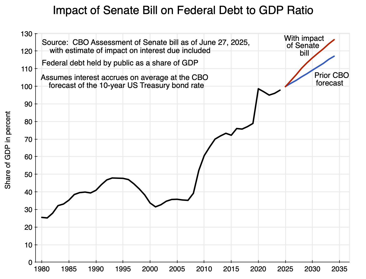
The resulting path for the federal debt to GDP ratio is shown in the chart at the top of this post, with the debt to GDP ratio shown going back to 1980 to provide context.  For the 2025 to 2034 period, the curve in blue shows what it would be under the prior (January 2025) CBO forecast (which assumed current law would be followed), while the curve in red shows what it would be if the Senate bill is passed and then approved also in the House and signed into law by Trump.

The federal debt to GDP ratio (defined as the net federal debt held by the public, where internal trust fund and other accounts – such as for Social Security – are netted out) is now close to 100% of GDP.  It was already on a rising path in the prior (baseline) CBO forecast released in January (a forecast based on budget and tax law as it stood at the time).  With the Senate bill it will now rise even faster.  Fiscal deficits will soon exceed 7% of GDP under Trump – unprecedented in times of full employment other than during World War II – and the federal debt to GDP ratio will soon exceed the record set in 1946 when it hit 106% of GDP.  Under the Senate bill, it is expected to exceed 106% of GDP by 2027, and will reach 126% of GDP by 2034, with no sign of it falling from there.

One should also note that the CBO forecasts of GDP and the federal deficit are long-term, and of necessity the CBO can only forecast some long-run path of steady growth.  In reality, of course, there will be fluctuations around any such path; it is just impossible to know when.  But when there is a downturn (and it is a matter only of when, not whether, with that likelihood especially high due to the chaos of the Trump administration), the fiscal deficit will rise and should rise.  The federal government has an important responsibility to help stabilize the economy.  But that higher fiscal deficit will add to federal debt, and the federal debt to GDP ratio will be higher following any such downturn even when GDP has returned (hopefully) to its previous long-term path.

The CBO forecast of the debt to GDP ratio in the outer years is therefore likely to be an underestimate.  By 2034, it could be a good deal higher than 126% of GDP unless Republicans in Congress finally recognize that their cuts in taxes are irresponsible.

In addition, not only are the measures included in the “One Big Beautiful Bill” tremendously costly, they will only be of benefit to those with higher incomes.  Based on the earlier version of the One Big Beautiful Bill (HR1) passed by the House in May, the CBO estimates that the lowest three deciles of households will see their absolute incomes (post taxes and transfers) reduced.  The CBO issued its estimates for this bill on June 12.  It is not clear whether the CBO will do a similar analysis for the specific Senate bill now being considered, and if so when it would come out.  However, the primary measures in the House and Senate versions of the bill are similar, and the distributional impacts will likely be similar.

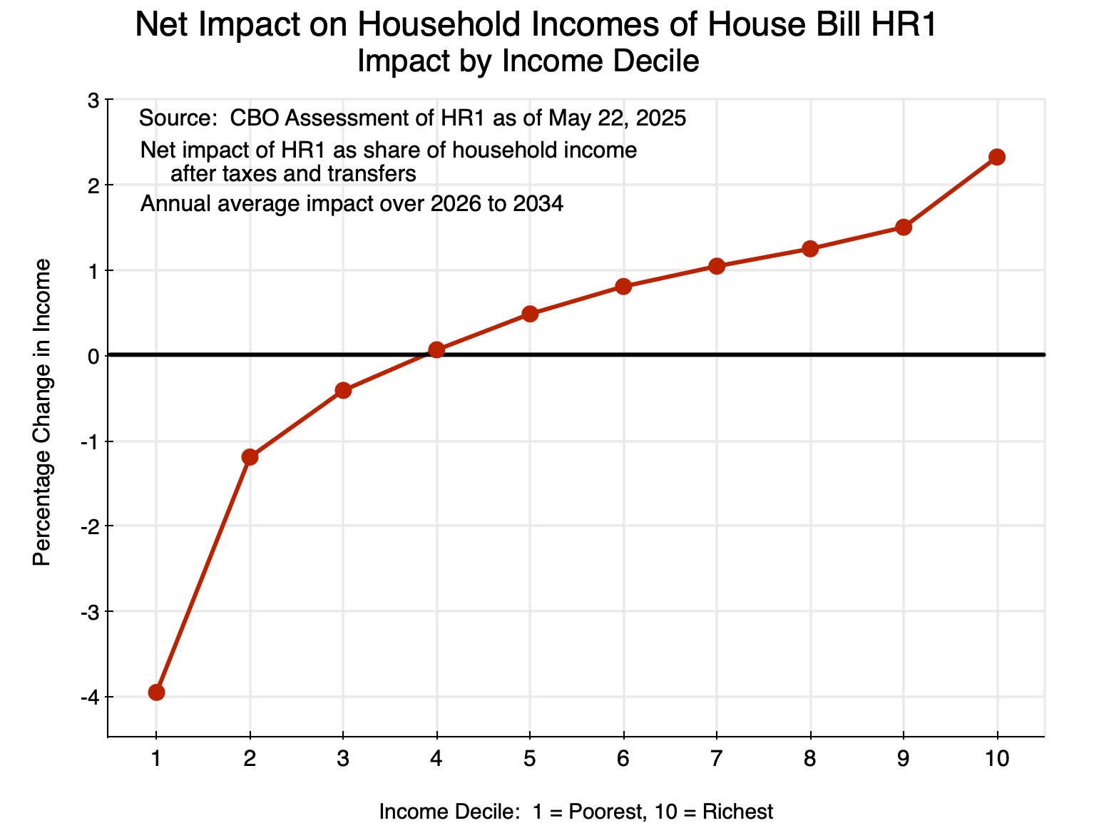
The CBO estimates of the impacts on households by decile of income of the version of the bill passed by the House (as a percent of household incomes) were:

Chart 2

The poorest decile of households would be especially adversely affected.  They would lose 4% of their incomes in absolute terms, with this is in a bill that is being funded primarily by increased federal borrowing.  Households in the second and third deciles would also lose in absolute terms, while those in the fourth decile would see (on average) almost no impact.  Higher income households then gain progressively more, with especially large gains for the richest (highest decile) households.  Note that this is presented as percentages of household incomes, after taxes and transfers.  Since incomes are much higher for the highest income households, the absolute dollar gains are especially high for the richest households.

There has never before been such an expensive and highly regressive measure passed by Congress.  But it appears this bill will soon be passed and signed into law by Trump.

The Impact of Covid-19 on Mortality

Chart 1

Chart 2

A.  Introduction

As a diversion from the more strictly economic posts usually on this blog, this post will examine data that can be used to better understand the impact the Covid pandemic had on US mortality rates.  The Social Security Administration provides figures each year on historical mortality rates as part of the legislatively mandated Annual Report of the Board of Trustees of the Social Security Trust Funds.  The 2025 Trustees Report was released on June 18, and as part of the background material, it provides mortality rates by year of age (for males and for females) for the year 2022.  Prior Trustee Reports provide the figures for earlier years (always with a three-year lag).  Comparing the mortality rates of one year to another allows us to see the impact of an event such as the Covid pandemic.

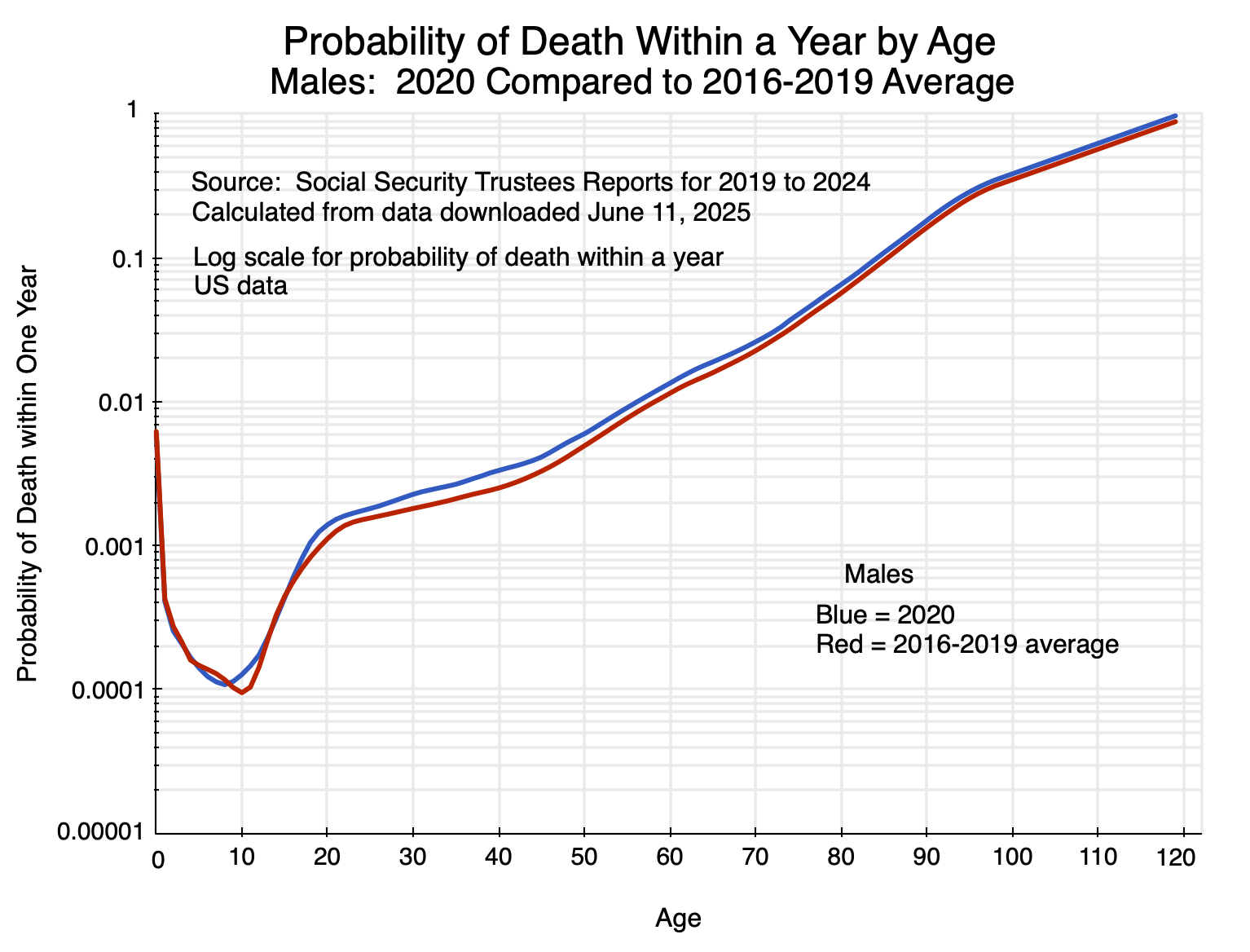
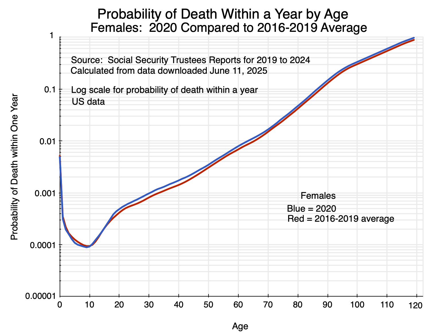
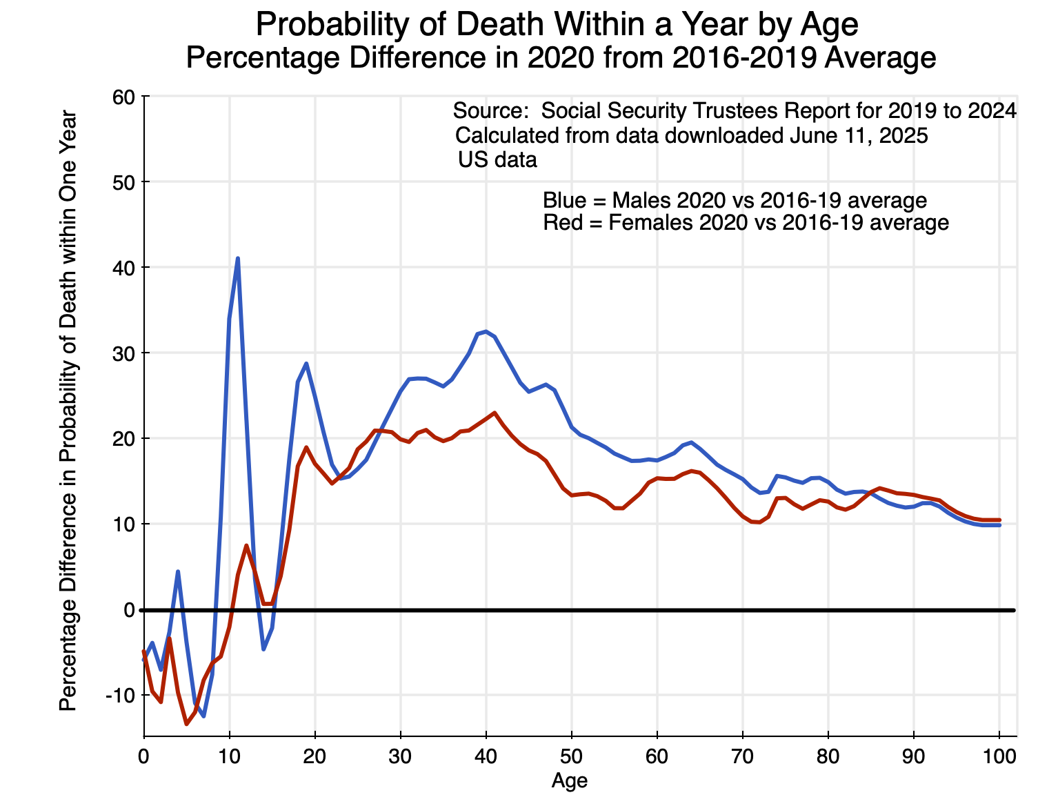
The charts above show the probabilities of dying within a year in 2020 (the first year of Covid) for someone of a given age compared to what it was on average over 2016 to 2019.  The gap between the respective curves is a measure of the impact of the special circumstances of 2020 compared to what would have been expected based on past experience.  One can look at such figures in different ways, which provide alternative perspectives.  As will be discussed below, in terms of the absolute difference in mortality rates (i.e. in percentage points), the impact was greatest for the elderly.  In terms of the relative difference in mortality rates (i.e. as a percentage of what they were in prior years), the impact was greatest on those in middle age – in their 30s and 40s.

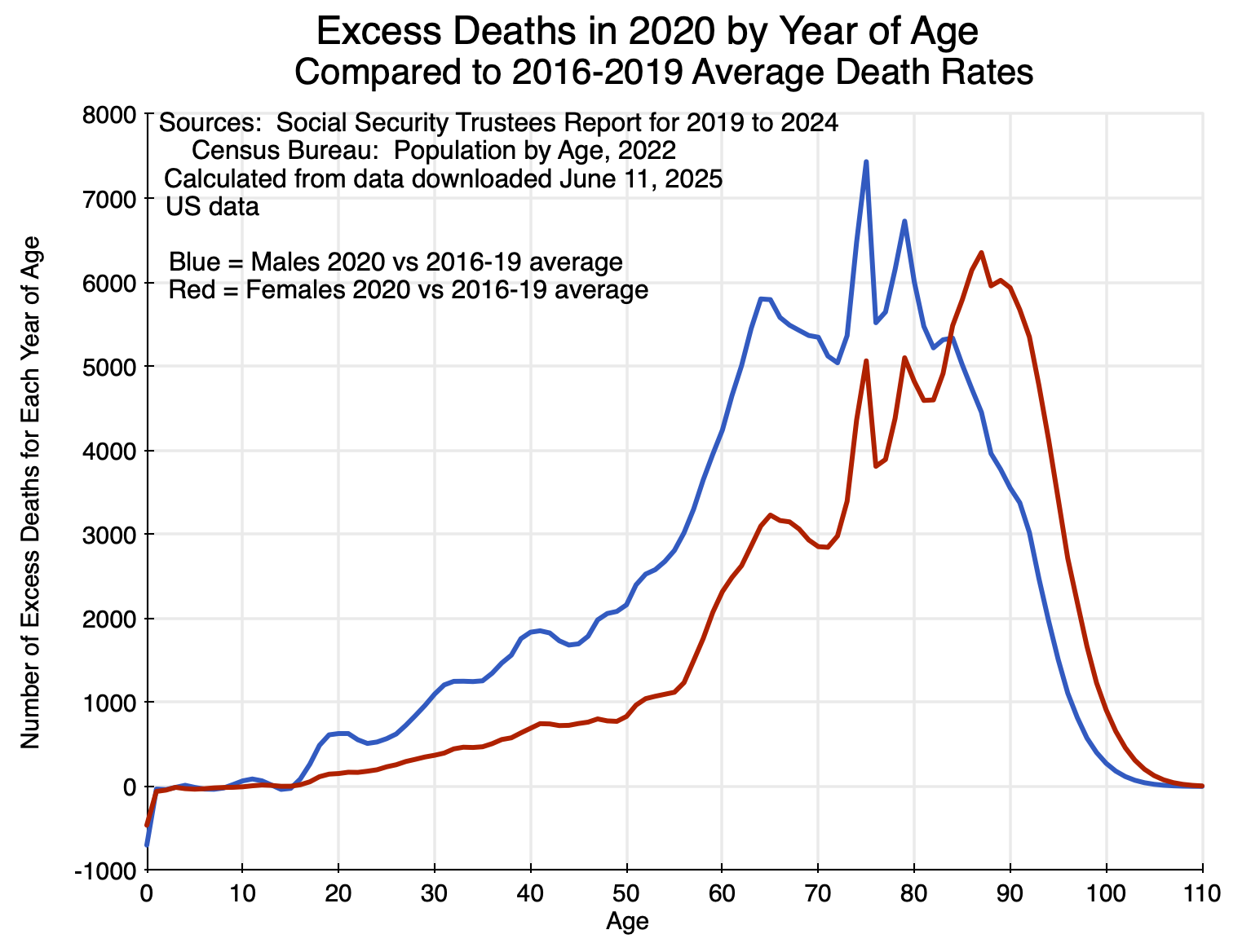
The data can also be used (together with data from the Census Bureau on population by age) to calculate the number of “excess deaths” due to the special circumstances of 2020 (and similarly for 2021 and 2022).  This impact will depend on the combination of the greater likelihood of dying combined with the population in each age group.  We will see that from this perspective, the impact (the number of excess deaths) was greatest for those in their 60s to their early 90s.

Also of interest (and indeed what first led me to look at these patterns) are the basic figures on mortality rates themselves by year of age.  Before seeing such figures, I would have guessed that mortality rates did not rise by all that much between the ages of 20 and 60 or so.  After that they would be higher, and I would have guessed progressively higher at an accelerating rate for those who were older.

But they do not follow such a pattern.  Rather, while the mortality rates rise with age, they rise at a remarkably steady rate from around age 20 to age 70 – basically doubling with each decade of life.  They then accelerate for those in their 70s to 90s (roughly tripling with each decade, up from doubling), before decelerating – although still increasing – for those older than around 95.

I found this pattern remarkable.  While I am an economist and not a biologist, I suspect that this pattern (with mortality rates doubling each decade up to around age 70), reflects something profound in how our biological systems function.

This pattern of mortality by age will be discussed in the first section below.  The section following will then look at charts similar to that for 2020 above but for the 2021 and 2022 figures.  The same basic pattern holds.  While deaths due to Covid diminished in 2022, they remained significant in that year (based on CDC estimates on deaths due to Covid), before dropping sharply in 2023 and by more in 2024.  The section will examine the percentage and percentage point differences in the mortality rates by age, focusing on the 2020 data.  It will then look at excess deaths by year of age in 2020 – as well as the totals for 2021 and 2022 – compared to what they would have been at the 2016-2019 average mortality rates.  The estimates calculated here of excess deaths in 2020 – and especially in 2021 and 2022 – are remarkably close to the CDC estimates on deaths due to Covid in those respective years.

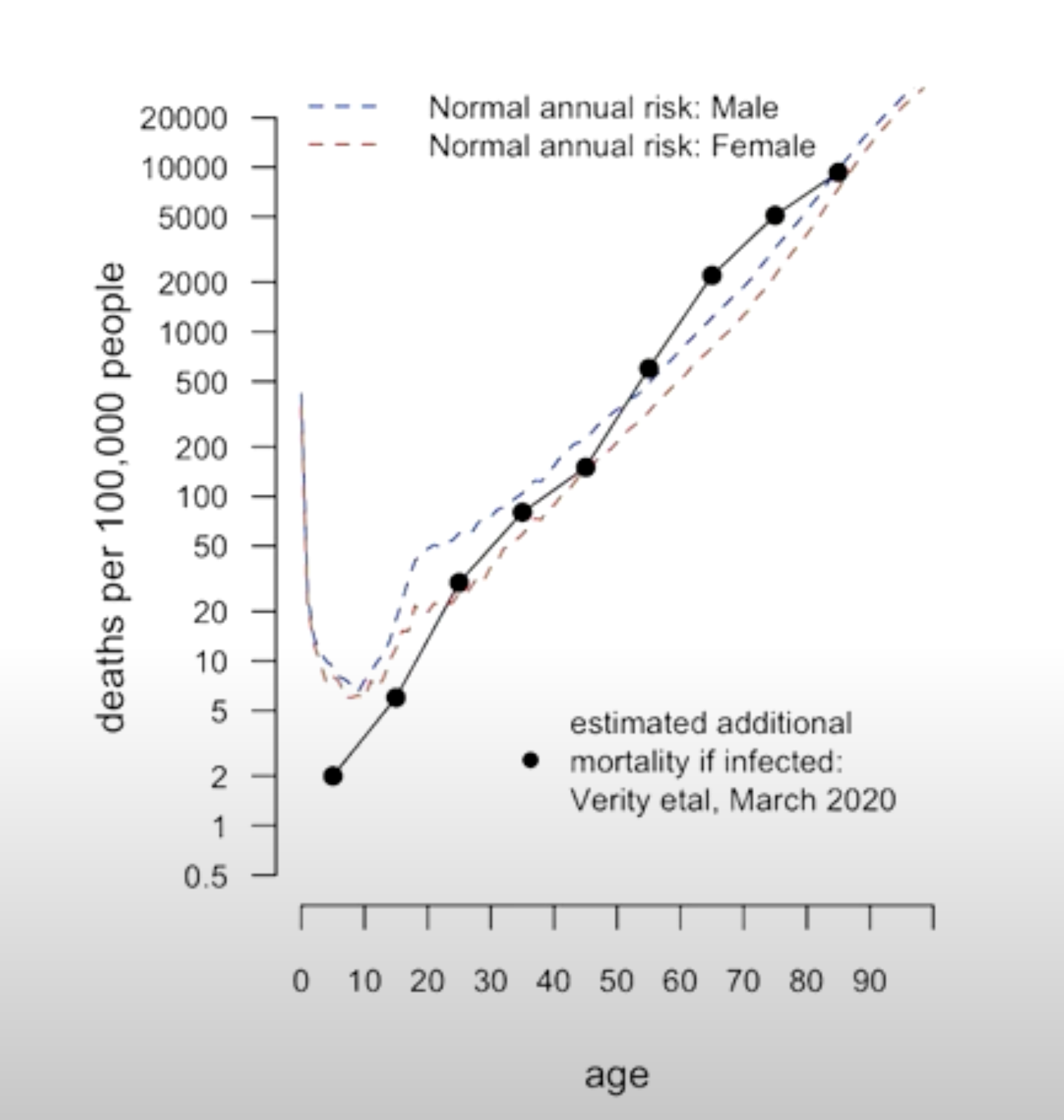
An annex to this post will then briefly examine material from a presentation by Sir David Spiegelhalter on the impact of being infected with Covid on death rates.  He compared them to pre-Covid death rates by age (based on UK data).  It was this work by Spiegelhalter that led me to look at US data on mortality rates.

Spiegelhalter found that the death rates by age were similar to the death rates of those infected with the virus that causes Covid.  That is, for those infected by the virus, the likelihood of dying due to Covid was similar to the likelihood of dying (pre-Covid) due to any cause within a year.

This was then grossly misinterpreted in the press.  As Spiegelhalter noted to his great dismay, instead of recognizing that this evidence pointed to a Covid infection as doubling the likelihood of dying within a year, the chart was interpreted by some in the press as saying the likelihood of dying within a year was the same whether or not one had come down with Covid.

The episode illustrates well how basic (and in this case highly important) statistics can be easily misinterpreted.

B.  Mortality Rates by Age

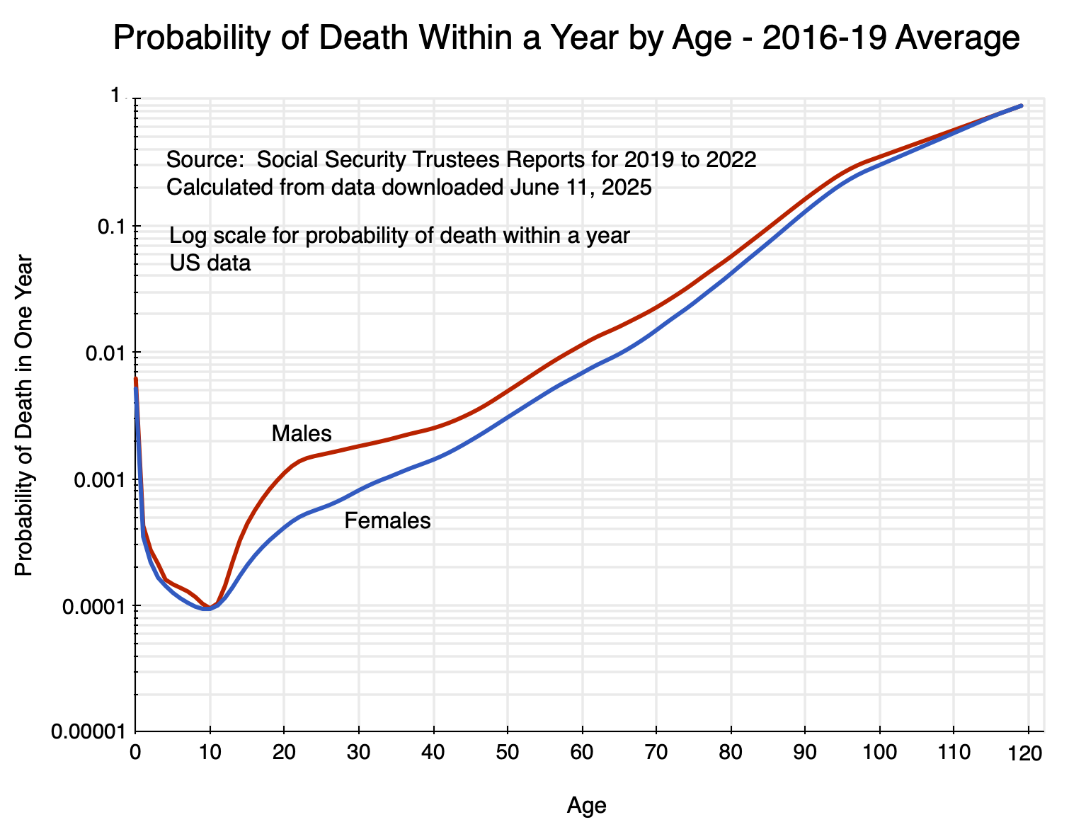
To start:  consider the basic pattern of mortality by age.  For males and for females, and using the 2016-2019 average (although any year could have been used for illustrating the basic pattern), the figures are:

Chart 3

The chart shows the probability of dying within a year for someone of a given age, with the vertical scale in logarithms.  It reaches a trough of around just 0.0001 ( = 0.01%) at around age 10 (following substantially higher rates as an infant, and especially for those in the first year after birth).  It then rises until the probability approaches 1 at the upper end.  The Social Security figures go all the way out to 120, but this is a modeled extrapolation as few are alive beyond age 110.

The death rates for males are uniformly above those for females.  They are especially higher at around age 20, and then remain higher (although at a diminishing proportion) until the age of 100 or more.  The higher rates for males are in part due to higher deaths for males from accidents, violence, and suicides.  For this reason, it is better to focus on the female rates to get a sense of the basic biological processes leading to the observed mortality rates.

As one may remember from their high school math, a straight line in a chart with a vertical scale in logarithms will follow a constant rate of growth, with the slope of that line giving the rate of growth.  In the chart above, the mortality rate for females rises at a remarkably steady rate (i.e. along a straight line) from age 20 to around age 70.  From the underlying mortality figures by age, one can calculate that the rate basically doubles (i.e. increases by about 100%, plus or minus around 20%) every decade over that age span.  The rate accelerates (the slope becomes steeper) from age 70 to around 95 – roughly tripling with each decade rather than doubling – after which it slows (as eventually it must:  the probability can never exceed 100%).

The mortality rates start, of course, at very low levels.  As noted above, the rate of dying within a year at age 10 (males or females) is only 0.0001 ( = 0.01%).  For females at age 20, it is around 0.0004 ( = 0.04%).  It then doubles to 0.0008 ( = 0.08%) at age 30, almost doubles again to 0.0014 ( = 0.14%) at age 40, basically doubles again to 0.0031 ( = 0.31%) at age 50, again to 0.0069 ( = 0.69%) at age 60, and again to 0.0150 ( = 1.5%) at age 70.  The pace then rises (roughly tripling with each decade) between ages 70 and 95 before slowing down.

The mortality rates before age 70 are all low, of course.  But it is interesting that they basically double each decade from age 20.  I suspect that this represents something fundamental about how biological systems function.

In any case, we can now look at how those mortality rates were affected by the special circumstances of 2020 (as well as in 2021 and 2022) during the height of the Covid pandemic.  Mortality rates rose, but far from uniformly by age.

C.  Mortality Rates in 2020, 2021, and 2022

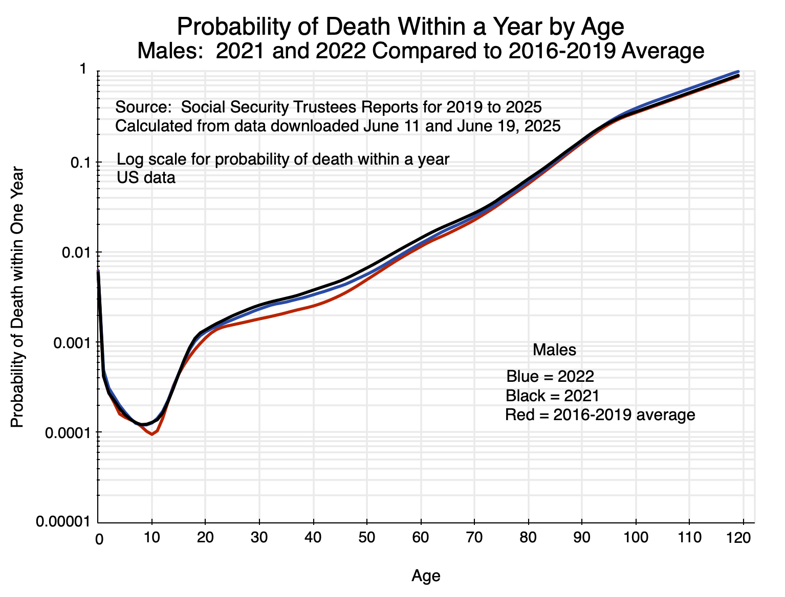
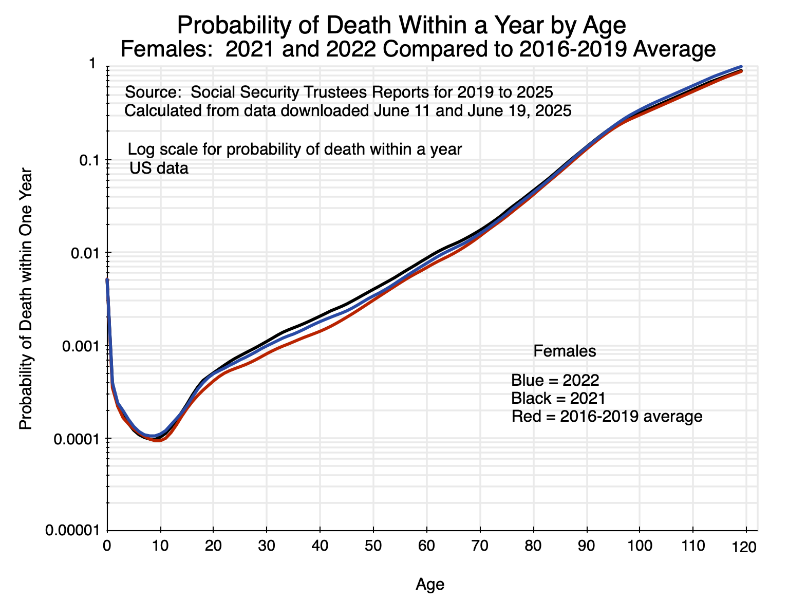
Charts 1 and 2 at the top of this post show what mortality rates were according to age for males and females, respectively, in 2020 compared to the average over 2016 to 2019.  The charts are similar for 2021 and 2022:

Chart 4

Chart 5

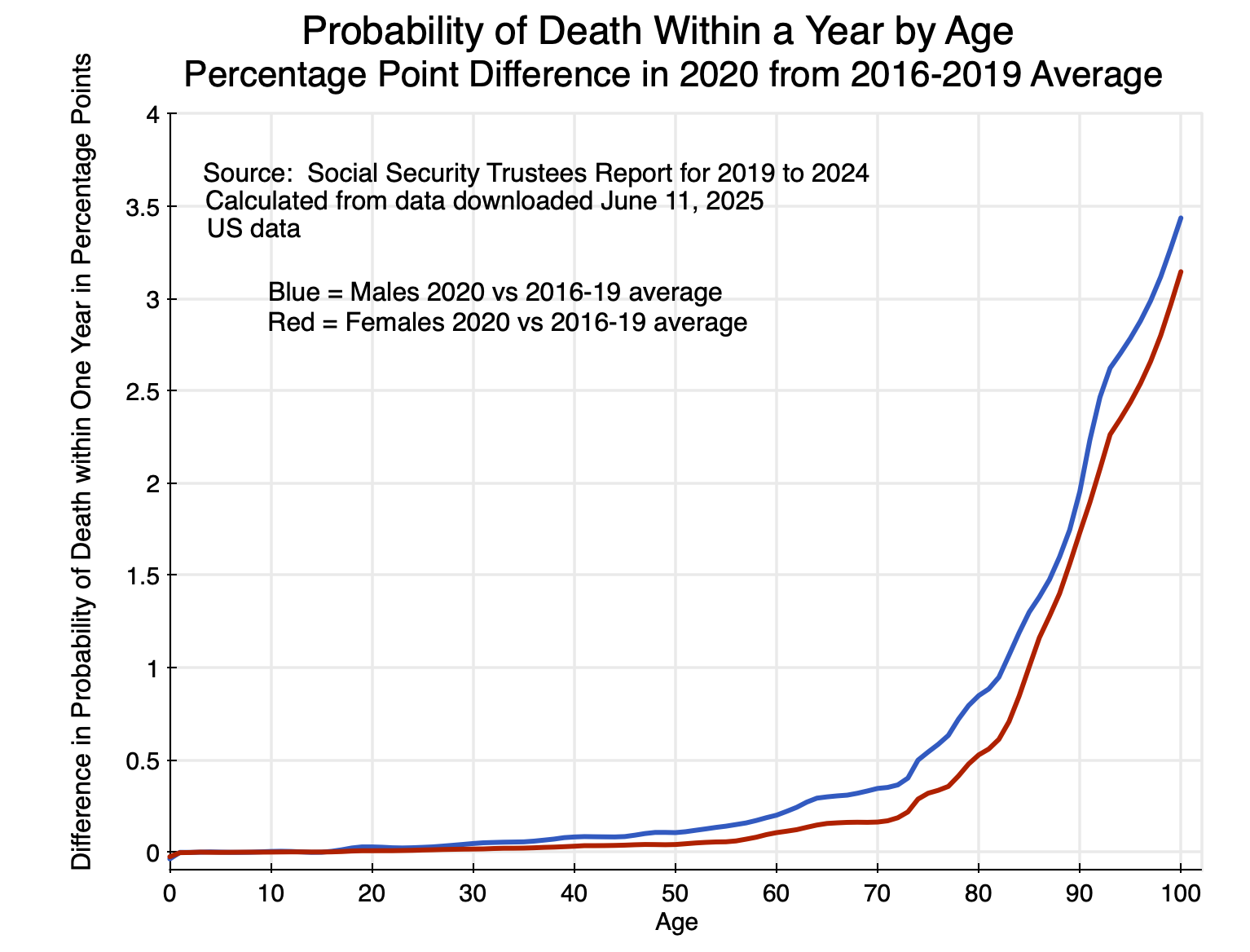
The gap between the lines shows the impact of the special circumstances of the respective years relative to pre-Covid mortality rates.  One can look at this gap in different ways.  Most commonly, the differences in the mortality rates have been shown in absolute terms (i.e. in percentage points).  That impact is greatest for the elderly.  For 2020 compared to the 2016-2019 average rates (the basic pattern is similar for 2021 and 2022, although at a different level):

Chart 6

The increase in mortality rates in 2020 relative to what they were before was far higher in absolute terms (i.e. in percentage points) for the elderly than for the young.  They were also consistently higher for males than for females.

And the differences by age are huge.  Keep in mind that the impact on mortality depends on a combination of the likelihood of being infected by the virus that causes Covid, and the likelihood that one will die if infected.  Based on these figures for 2020 compared to the average mortality rates between 2016 and 2019, the increase in mortality of males at age 90, say, was 1.95% points.  The increase for males at age 20 was, in contrast, 0.028% points.  That is, the increase was 70 times higher for males at age 90 compared to those at age 20.  For females, the increase was even greater:  almost 250 times higher for those at age 90 compared to those at age 20.  The impact of the 2020 events on the elderly was huge.

A different way to look at the figures is in terms of the percentage increase in mortality rates for someone of a given age.  For 2020 compared to the 2016-2019 averages (where again, the basic pattern is similar for 2021 and 2022):

Chart 7

In terms of the relative increase in mortality rates, the impact of the 2020 events was highest for those between the ages of 20 and 50 (along with a peak at ages 10 and 11 for males).  The absolute increase in mortality rates for those in this age range was not high (as seen in Chart 6).  But relative to the normally small probabilities of dying for those who are young or middle-aged, the relative increase was greater than for the elderly.

From this, coupled with figures from the Census Bureau on the US population for each year of age, one can calculate the number of “excess deaths” arising due to the special circumstances of 2020 (Covid and its indirect as well as direct effects), compared to what the mortality would have been at the mortality rates of prior years (where the 2016 to 2019 average was used as this base).

For 2020, the excess deaths by year of age were:

Chart 8

The impact was largest on the elderly, and especially so for females more than for males.  Up to age 15 or so, there was almost no impact.  Indeed, the data indicate that for those in their first year of life, excess deaths were substantially reduced.  There were then very small effects – some positive and some negative – up to age 15.

Adding up the number of excess deaths across all ages – and with similar calculations for 2021 and 2022 – leads to:

Calculated Excess Deaths CDC Covid Deaths % difference
2020 418,076 385,676 8.4%
2021 467,992 463,267 1.0%
2022 245,081 247,196 -0.9%
2020 to 2022 1,131,150 1,096,139 3.2%

The CDC estimates of deaths due to Covid by year are shown in the second column of the table.  The two estimates turn out to be remarkably similar, especially for 2021 and 2022 where they are within +/- 1% of each other.  And the methodologies are completely different.  The CDC figures are based on death certificate data reported to it for its National Vital Statistics System.  The excess death figures here are calculated from a comparison of mortality (by year of age) in each year compared to what the mortality rates were on average between 2016 and 2019, applied to Census Bureau figures on the US population by year of age in each of these years.

This surprising congruence might be a coincidence – although the figures are extremely close in two of the three years so it would have to be an extreme coincidence.  And while this is speculation, the calculated excess deaths figure in 2020 – which is 8.4% higher than the recorded number of Covid deaths in that year – might reflect the special circumstances of the health care system (and especially of hospitals) in that year.  Due to the rapidly spreading virus that year and with no vaccine yet available, hospitals were crowded with patients being treated for Covid.  One avoided going to a hospital except under dire circumstances.  That led to patients with conditions that would have benefited from being treated at a hospital avoiding such care when they would have benefited from it, and consequent higher death rates.  While not a direct consequence of being infected with the virus that causes Covid, their higher mortality would have been an indirect consequence.

This indirect impact of Covid then largely went away in 2021 and 2022, as the Covid vaccine led to lower case loads, less hospital overcrowding, and less reason to avoid going to a hospital when needed for non-Covid reasons.

D.  Conclusion

The Covid-19 pandemic was a tragedy.  Over 1.2 million Americans have died, which is more than double the number of American soldiers who have died in combat in all of the country’s wars since 1775.  The Trump administration terribly mismanaged the response to the then spreading pandemic in the first half of 2020, with Trump asserting that his bans on travel – first from China, later from Europe and elsewhere – would stop the spread of the virus and that it would soon “go away”.  It did not.  And by his statement that he would not wear a mask in public despite the CDC recommendation to do so, Trump made the refusal to wear a mask into a sign of political fealty.  This later carried over into a refusal to be vaccinated.

This had real consequences.  People died.  And they died at higher rates in proportion to the share of the vote in a state for Trump.

Management of the Covid pandemic would have been difficult by even the most capable of administrations.  But it was not capably managed in the US.  As a reasonable comparator of what should have been possible, one can consider the case of Canada.  Deaths from Covid in Canada were 1,538 per million of population (as of April 2024, when cross-country comparable data collection stopped).  For the same period, it was 3,642 per million of population in the US:  2.4 times as high as in Canada.  If the US had had the same mortality rate as Canada, deaths would not have been 1.2 million (as of the end of 2024), but rather about 500,000.  An additional 700,000 Americans would be alive today.

The virus that leads to Covid will now be with us for the foreseeable future.  The peak number of deaths came in 2021 as it was the first full calendar year when the virus had spread to all parts of the nation.  In 2020, there were very few cases nationally until mid-March, and it did not spread to all corners of the nation until several months later.  Vaccines became available in 2021, but were in short supply for most of the first half of the year.  And even when fully available without restriction, a substantial share of the population refused to be vaccinated.

But with the vaccinations in 2021, as well as the immunity obtained by those who were infected by Covid at some point and survived, the number of deaths from Covid fell by almost half in 2022 to 247,000 in the CDC data.  See the table above.  Deaths then fell further to 76,000 in 2023 and to 47,500 in 2024.  Deaths in the coming years will likely be in the tens of thousands each year, similar to the pattern seen for deaths due to the influenza (flu) virus.  On average, about 30,000 have died each year since 2011 from influenza, but this has varied widely from a low of 6,300 in the 2021/22 season (when measures taken by many to limit exposure to Covid also served to limit exposure to the flu virus) to a high of 52,000 in the 2017/2018 season.  Deaths from Covid-19 may be similar in the coming years, with a good deal of variability and levels that depend on measures such as how many will be vaccinated each year against the evolving variants of the virus.

Mortality rates will also vary by age.  While the variation by age may be moderating, it is likely that the elderly will remain the most severely affected in absolute terms (as in Chart 6 above).  However, one should still recognize that in relative terms (relative to mortality rates at the given age), those in middle age may well remain the most affected (as in Chart 7 above).

Covid-19 was a tragedy.  There is, unfortunately, little indication that the mistakes that were made in the management of it will not be repeated when the next pandemic comes.


——————————————————————————————————-

Annex:  Mortality Rates by Age from Infections by Covid Compared to Pre-Covid Mortality Rates from All Causes 

The impetus for this post came from a chart I saw in a video of a November 2021 lecture by Sir David Spiegelhalter (a professor at the University of Cambridge, and on the board of the UK Statistics Authority).  See the section starting at around minute 18.  Based on very early (March 2020) UK data on the Covid fatality rate (later confirmed with much more data), he showed that the fatality rate if infected by Covid was similar for any given age as that of dying for any reason (before Covid began to spread) at that age.  The chart, with the vertical scale in logarithms, was:

Chart 9

Two points to note:

a)  Leaving aside the impact of a Covid infection, the mortality rate (from all causes, pre-Covid) in this UK data rises with age (from around age 10) at a remarkably steady rate through to age 90.  As noted in the post above, I was surprised that the pace at which mortality increases with age is close to the same for those in their 20s and 30s as it is for those much older.

b)  The mortality rate of those infected with Covid was basically the same as the mortality rate pre-Covid.  That is, being infected with Covid basically meant that the mortality rate doubled for any given age.  Note that this is not the same as what is in Chart 7 above, which shows the increase in the mortality rate for any given age in 2020 during the Covid pandemic.  Those increases were in the range of 20 to 30% for those in their 30s and early 40s, declining to 10 to 15% for the elderly.  It is not the same in Chart 7 because not everyone caught the virus that causes Covid in 2020 (and was also US rather than UK data, although this was probably not a factor).  Chart 9 from Spiegelhalter shows mortality rates from Covid for those who were infected with the virus that causes it.

Spiegelalter’s finding was then profoundly misunderstood.  Some in the British news media were soon citing this as “evidence” from a highly esteemed scholar that said (as in a headline in The Sun newspaper):  “Your risk of dying is NO different this year – despite coronavirus epidemic, says expert”.

Spiegelhalter was not saying that at all.  He had thought the correct interpretation would be obvious, but clearly it was not.  The chart is saying that, at each age group, the likelihood of dying if infected with the virus that causes Covid is close to the same as dying at that age for any reason (pre-Covid).  Hence, if you have been infected by Covid, your probability of dying that year has doubled.  As Spiegelhalter later noted, this is a good example of how statistics can be easily misinterpreted.

(After Spiegelhalter complained, the Sun changed the title to:  “Your risk of dying from coronavirus is roughly the same as your annual risk, says expert”.  A bit better, but still easy for readers to misinterpret.)

Imports Do Not Subtract From GDP: Econ 101

Chart 1

A.  Introduction

Trump has undermined what had been a strong US economy more quickly than most expected.  The BEA released on April 30 its initial estimate (what it labels the “advance estimate”) of the growth in GDP in the first quarter of 2025.  The economy contracted by 0.3% at an annual rate.  Real GDP grew at solid – indeed excellent – rates while Biden was in office.  The economy grew by 6.1% in 2021 as it emerged from the Covid crisis – faster than in any year since 1984 – and by 2.5% in 2022.  It then grew at a rate of 2.9% in 2023 and 2.8% in 2024.  While the GDP estimate for the first quarter of 2025 will be revised as additional data becomes available in the coming months, this is a terrible start for the new administration.

The cause of this fall in GDP in the first quarter of the Trump administration has been misinterpreted by many.  Prominent among them was Peter Navarro, the primary trade advisor in the White House.  In an interview on CNBC, Navarro asserted:

“when you strip out inventories and the negative effects of the surge in imports because of the tariffs, you had 3% growth.”

No:  Output did not grow.  It fell at a 0.3% rate.  There was indeed an extraordinary surge in imports.  Trump began to impose major tariffs on imports soon after taking office, with a promise of far higher rates to come.  And indeed, on April 2 he announced extraordinarily high (and highly variable) tariff rates on every “country” in the world (including one occupied only by penguins), only to back down on April 9, saying they would be postponed for 90 days.  In anticipation of what might come, imports of goods and services rose in the first quarter of 2025 at an astounding 41% annualized rate and imports of goods only (which can be stored) rose at a 51% rate.

But an increase in imports does not – in itself – affect the calculation of GDP.  GDP is a measure of domestic production (that is what the D stands for in GDP:  Gross Domestic Product).  Domestic production is what it is in the accounting regardless of how much is imported.

The confusion of Navarro and many in the news media stems from the formula that all are taught in an introductory Econ 101 macroeconomics class:

GDP = Consumption + Fixed Investment + Investment in Inventories + Exports – Imports

(where government consumption and investment can be combined with private consumption and investment, which we will do here for simplicity).  Imports are subtracted out at the end of this formula because Consumption, Fixed Investment, Investment in Inventories, and Exports all include the imports that help supply (directly or indirectly) these components of demand.  That is, Consumption (for example) includes consumption of domestic production as well as consumption of whatever is imported and used for that purpose.  And similarly for the other demand components.  Total Imports must then be subtracted out (as it is at the end of the formula) to arrive at what domestic production was.  That domestic production is GDP.

While it is easy to see why there would be such a mistake in the interpretation of how GDP is determined, there is no excuse for policy officials as well as journalists who write on economic issues to make such a mistake.

I have discussed before on this blog how GDP is estimated (see here and here).  But given this widespread misinterpretation of the 2025Q1 figures, it is worth reviewing the issue again.  That will be covered in the first section below.  The section that follows will then discuss the new GDP estimates themselves, and what those figures are telling us about how the economy has responded to the new Trump administration.  This concrete example will also help to reinforce the understanding on how imports enter.

The concluding section will then briefly look at what is in prospect for the GDP figures, both in the coming months and beyond.  While the economy is probably not yet in a recession, the policies of the new Trump administration (and its chaotic implementation) make it increasingly clear that the US will soon enter into a recession, unless Trump quickly reverses what he is doing.  And there is little likelihood of Trump doing that.

B.  Econ 101:  What GDP Means and How it is Estimated

Numerous news sources (as well as the official White House press release) misinterpreted the impact of imports on the GDP estimate for the first quarter of 2025.  As one example among many, the CNBC report on the GDP figures stated:

“Imports subtract from GDP, so the contraction in growth may not be viewed as negatively given the potential for the trend to reverse in subsequent quarters. Imports took more than 5 percentage points off the headline reading.”

Which is wrong.

GDP is an acronym for Gross Domestic Product.  “Product” means what is produced; “Domestic” means what is domestically produced; and “Gross” refers to the gross level of investment being counted rather than investment net of an estimate of depreciation (the latter measure of investment would then lead to Net Domestic Product, or NDP).

So how is GDP estimated?  As was discussed in the earlier blog posts referred to above, the BEA (the government agency that produces the GDP accounts) does this in three different ways.  In principle, all three should lead to the same estimate for GDP.  Because they are all estimates based on surveys and other statistics, they don’t although they should be close. There will always be statistical noise, and the three different estimates serve as a good check on each other to help find whether a mistake was made somewhere.

One approach is to estimate domestic production directly – sector by sector.  However, data for this is the most difficult to come by, and the first BEA estimate of GDP by this method is only provided three months after the end of a calendar quarter, i.e. in late June for the January to March quarter.  A second approach is to estimate domestic production by the incomes generated.  Since whatever is produced and sold will be reflected in incomes (in the wages of the workers employed, and then in the profits that remain following the payments for all the inputs used in production plus the wages paid), this should in principle also sum to GDP.  The BEA provides its first estimate of GDP using this approach (which, to limit confusion, it labels Gross Domestic Income, or GDI) two months after the end of a calendar quarter, i.e. in late May for the January to March quarter.

The third approach – and the one most commonly considered when GDP is referred to – is to estimate GDP from the uses of whatever is produced.  Whatever is produced is used, and if those uses can be estimated, this can be used to arrive at an estimate of what is produced, i.e. GDP.  The BEA can also provide a reasonable estimate of GDP this way relatively quickly after the end of each calendar quarter.  It issues its initial estimate one month after the end of each calendar quarter, i.e. in late April for the January to March quarter.  While the estimate will be revised as more data become available in the subsequent months, it is this estimate of GDP that receives the most attention as it is the first to be released.  Keeping track of the various demands for production is also important in a modern economy since we know from Keynes that production (up to a limit set by full employment) will largely follow from what the demands are.

This estimate is also built around the well-known equation referred to in the introduction above.  Starting with the simplest form in order to make clear that GDP is a measure of domestic production and not of demand, consider an economy where there is no foreign trade.  The equation is then:

GDP = Consumption + Fixed Investment + Investment in Inventories

The final uses of (the final demands for) goods and services are that they are either consumed or invested.  But what is consumed or invested in a period will normally differ from what is produced.  The simple trick, then, is to include along with the final demands the amount that is added to inventories (if production exceeds the sum of the final demands in the period) or taken out of inventories (if production falls short of the sum of the final demands in the period).  Hence by adding the net change in inventories (inventory accumulation, which is an investment) to the final demands for goods and services, one will arrive at what was produced in that period.  (Note that the terms “additions to inventories”, “investment in inventories”, and “accumulation of inventories” all refer to the same thing and are used interchangeably.)

Simple, although it can easily lead to the mistake of treating the demand for goods and services as GDP, when GDP is in fact the production of goods and services.

We can add foreign trade in goods and services to this.  There will be exports (also a final demand for goods and services) as well as imports.  Imports are an additional source of supply of goods and services that add to what is domestically produced.  Putting the supply of goods and services on the left and the demand for goods and services on the right, one has:

Supply of goods and services = Demand for goods and services

GDP + Imports =  Consumption + Fixed Investment + Investment in Inventories + Exports

The supplies of goods and services – whether from domestic production (GDP) or foreign production (Imports) – are used to meet the final demands for Consumption, Investment, and Exports, along with any accumulation of inventories if the total supplied exceeds the final demands (or decumulation of inventories if final demands exceed supplies).

Moving Imports to the right side of the equation, one then has the well-known:

GDP = Consumption + Fixed Investment + Investment in Inventories + Exports – Imports

It is important to keep in mind that imports typically enter indirectly, as an input to what is being produced and thus enabling a greater overall supply.  But one cannot map what share of Consumption, say, came from domestic supply and how much from foreign supply.  Imports are a resource that enables the nation to provide more.  How can one know, for example, whether a gallon of fuel, say, that was imported was used to help produce an item for consumption, or an item for investment, or an item for exports, or was added to inventories?  And even if the imported item can be individually identified, the complex nature of multi-level production (where intermediate goods produced can be used for a variety of different final goods) often makes it impossible to trace what an imported item ended up being used for.

As a result, the BEA cannot produce individual estimates of how much of Consumption, say, came from domestically supplied items and how much came from items produced with imports as a resource.  All it can provide are estimates of each of the demand components (including any addition to – or subtraction from – inventories), and then subtract total imports from the total demands to arrive at an estimate of what domestic production (GDP) was.

Imports in this accounting thus do not subtract from GDP, even though numerous news sources (and Trump officials) asserted precisely that.  If imports had been $1 billion higher, say, then there would have been $1 billion more in Consumption, or in Fixed Investment, or in Investment in Inventories, or in Exports (or some combination).  Subtracting that extra $1 billion at the end of the equation then leaves GDP exactly the same.

This is all accounting, or as economists refer to it, national income accounting.  Domestic production – GDP – did indeed fall at an annual rate of 0.3% in this initial estimate of GDP for the first quarter of 2025.  This was a sharp reduction from the strong and steady growth the country had enjoyed under Biden.  The country had nothing close to “3% growth”, as Peter Navarro wrongly asserted.

The figures for GDP and the components of demand that sum to GDP nevertheless acted in highly unusual ways in this first quarter of the Trump administration.  The next section of this post will examine those.

C.  GDP and Its Demand Components in the First Quarter of 2025

As noted before, the GDP estimates released by the BEA on April 30 are its initial or “advance” estimates of GDP and related figures in the National Income and Product Accounts.  Updated estimates based on more complete data will be provided with the second estimate in late May and again with the third estimate in late June. These estimates will likely differ to some degree from these initial estimates.

Historically, the average change in the estimated growth rate of GDP (in percentage points) from BEA’s advance estimate to its second estimate has only been 0.1% points, and also only 0.1% from the advance estimate to the third estimate.  But one has to keep in mind that those are changes on average, where sometimes the initial estimates are revised up and sometimes revised down.  The very small average difference (only 0.1%) means that there is little bias in the initial estimates historically:  they are as often revised up as revised down.  In absolute terms (i.e. ignoring whether the revisions were positive or negative), the average change from the advance estimate to the second estimate was 0.5%, and from the advance estimate to the third estimate was 0.7%.  Such changes are more significant, and there are even larger changes in periods when, such as now, the economy is going through major disruptions.

Due to the far from normal increase in imports resulting from uncertainty on what tariffs Trump will impose (which appear often to be based on a whim, and announced on social media posts), it is certainly possible and indeed likely that the GDP estimates for 2025Q1 will be revised by more than they normally have in the past.  Investment in inventory accumulation is especially difficult to estimate, and may see an especially large revision.

It is therefore quite possible that once revisions to the accounts are made based on more complete data, growth in real GDP will shift from the small negative (-0.3%) in the current estimate to possibly a small positive.  This should not, however, be viewed as terribly significant.  There is no chance that the revisions will bring growth anywhere close to the almost 3% rates the nation enjoyed under Biden in 2023 and 2024.  So while the analysis here has to be based on the figures released in the advance GDP estimates, the basic story should hold as the second and third estimates of GDP are released in the coming months.

This table summarizes the key figures:

Growth in Real GDP and Its Demand Components

2025Q1 vs 2024Q4 % change $ billion change
Real GDP -0.3%   -$16.2
Personal Consumption  1.8%   $72.4
Gross Fixed Investment  7.8%    $80.9
  o/w Information Processing Equipment 69.3%   $73.6
Investment in Inventories  $131.2
Government Expenditure -1.5%  -$14.6
  Federal Government -5.1%  -$19.8
    o/w Defense Spending -8.0%  -$18.0
  State & Local Government   0.8%     $4.9
Exports  1.8%   $11.6
Imports 41.3% $333.3
Seasonally adjusted annual rates; 2017 constant$

Starting from the top:  Domestic production in real terms (real GDP) fell at an annual rate of 0.3%.  In dollar terms (in constant 2017 prices) the fall was $16.2 billion.  This change in domestic production was far surpassed by the increase in imports (foreign production) of $333.3 billion in real terms, as individuals and businesses sought to get in front of Trump’s promised tariffs.

Much of the increase in imports likely went into the increase in inventories, which rose by $131.2 billion in real terms.  As discussed above, it is not possible to estimate for each of the demand components (the change in inventories being one) how much can be attributed to domestic supplies and how much to imported supplies.  It is likely, however, that with such a sizeable jump in imports (41.3% at an annual rate), a substantial share went into inventories.

But a significant share of the increase in imported supply was also used directly or indirectly for the final demand components of GDP.  As discussed before, each of these reflects the use of a combination of both domestic and imported supplies.  Take Gross Fixed Investment, for example.  It rose at the very fast rate of 7.8% in annual terms.  If one digs into the reported components for this, one will see (in Table 3 of the BEA release) that fixed investment in Information Processing Equipment rose by $73.6 billion in the quarter (69.3% at an annual rate).  That one component of investment accounted for over 90% of the overall increase in Gross Fixed Investment in the period (which was $80.9 billion).  Investment in Information Processing Equipment had not been booming before:  It in fact fell by $10.0 billion in the prior quarter, rose by $21.6 billion in the quarter before that, and rose by $9.7 billion in the quarter before that.

The highly unusual behavior in such investment in the first quarter of 2025 coincided with the uncertainty generated by Trump’s tariffs.  And Information Processing Equipment is the type of equipment that firms will often import directly and have installed.  It will thus count as part of Gross Fixed Investment in the GDP accounts.  Fixed investment rose in the first quarter of 2025, but it is likely that this primarily reflected a rush to import specialized equipment before even higher tariffs (whatever they will be) are imposed by Trump.

There was likely a similar factor that affected the Personal Consumption component, although to a lesser extent than what was seen for Fixed Investment.  Personal Consumption rose by 1.8% in real terms at an annual rate.  That is not all that high (it rose at a 4.0% rate in the fourth quarter of 2024 – the last quarter of the Biden administration – and by 3.7% in the third quarter of 2024).  But at least part of this would have come from businesses and individuals importing items before prices go up due to Trump’s tariffs.  Indeed, it is possible – and indeed likely – that net of what was imported to supply this demand (directly or indirectly), the domestic supply for Personal Consumption may well have decreased.  As a personal example, my wife and I decided to go ahead and buy now a new Apple iMac computer (which is assembled in China) for our home use.  Prices may soon skyrocket.  That purchase counted in the Personal Consumption category of the GDP accounts.

It is therefore a mistake to assert, as Trump officials did, that domestic production grew at a healthy rate.  The Navarro quote cited above refers to 3% growth, and the White House press release (that Navarro may have helped prepare) similarly says:  “Core GDP grew at a robust 3.0%.  This signals strong underlying economic momentum that occurred after President Trump’s inauguration.”  What they both appear to be referring to is what the BEA calls “Final sales to private domestic purchasers”.  It grew at a 3.0% rate.  It is defined as the growth in Personal Consumption and in Gross Fixed Investment together.  But as just discussed, much and possibly more than all of that growth reflected the surge in imports before tariffs go up.  Navarro (and others as well) do not realize that those items in the GDP accounts include imports.

The other items in the demand components of the GDP accounts did not change as much.  Federal government expenditures on goods and services (i.e. federal government consumption expenditures and gross investment) fell by $19.8 billion in annual terms (5.1%).  But this cannot be attributed to cuts pursued by Elon Musk and his DOGE group.  Of the $19.8 billion fall, $18.0 billion was due to a reduction in Defense Spending.  That has not been a DOGE focus.  Rather, with a change in administrations, decisions on payments and on new procurement contracts are often delayed as the new team comes in.

Finally, a technical note:  Some may have noticed that if one adds up the $ changes in the above table for Consumption, Investment, and so on in the well-known GDP equation, the sum comes to a dollar change of -$51.8 billion.  This is more than the reported fall of -$16.2 billion.  The reason for this difference is that the BEA uses chain-weighted price indices to deflate the nominal estimates of the GDP demand components.  (For a discussion of chain-weighted indices, in the context of how the CPI and Personal Consumption Expenditures – PCE – price deflators are calculated, see this earlier post on this blog.)

Chain-weighted price indices are based on weights derived from expenditure shares of individual items in the current period and in the prior one.  The BEA uses chain-weighted price indices for all the price deflators it calculates.  A property of chain-weighted price indices is, however, that a sum (such as real GDP here) will not necessarily be equal to the sum of the individual components (such as demand components here) in real terms.  The sum will in general be close, but the BEA warns readers that they will not be the same.

D.  Prospects and Conclusion

In the near term, and as noted above, the BEA will issue its second estimate of the GDP accounts for 2025Q1 in late May and its third estimate in late June.  It will then start the quarterly cycle again with its advance estimate of the GDP accounts for 2025Q2 in late July, and so on.

With the major disruptions to the economy due to Trump, there will likely be significant changes in a number of the figures when the second and third GDP estimates are released.  The import estimates will likely not be among them (despite the 41.3% jump in the period, or $333.3 billion) as the foreign trade accounts are fairly well known in real time (as imports are recorded as they go through customs).  But investment in inventories is much more difficult to estimate.  The BEA advance estimate is that they rose by $131.2 billion (in real terms), but I would not be surprised if, in the updated figures based on more complete data reports, inventory accumulation turns out to be higher.  If so, then the estimated growth in GDP will be higher.  If (purely for the sake of illustration – I am not predicting this), investment in inventories turns out to be $50 billion higher than shown in the advance estimate (i.e. $181.2 billion rather than $131.2 billion), and all else is the same as estimated now, then GDP would have grown at a +0.6% rate rather than fallen at a -0.3% rate.

A change of such a magnitude would not be surprising.  GDP growth would still be low, and far below the growth rates achieved when Biden was in office, but possible.  But the basic underlying story would remain that businesses urgently brought in imports out of concern (and great uncertainty) about how high tariffs might soon be.

The continued incoherence in Trump’s policies does not augur well for the economy for the rest of the year either.  This was demonstrated on April 2 as Trump announced (on what he called “Liberation Day”) his so-called “reciprocal tariffs” at rates as high as 50% (and higher for China).  Businesses were in shock, and it took some time before anyone could figure out how Trump’s rates had been set.  They were not at all reciprocal, but rather calculated based on the bilateral trade deficit of the US (for goods only, i.e. excluding trade in services) divided by US imports of goods from the country.  Trump then backed down a week later, and said he would postpone them for 90 days while a series of deals with countries were negotiated.

Businesses are now basically frozen.  They cannot decide on what investments to make – if any – as they cannot know what tariff regime they will be operating in.  They have also seen that Trump is more than willing to use the powers of the state to punish companies that upset him, and to take actions that are in blatant violation of the law (knowing that the judicial system takes time to act, and that once it does act they will be faced with a fait accompli).  A sound legal system that all must abide by – including a president – is fundamental to any modern economy.

Households are similarly wary.  Consumer expectations have plunged, and both the index of consumer sentiment of the University of Michigan and the Consumer Confidence Index of The Conference Board have dropped each and every month of Trump’s term in office from a peak in November/December 2024.  It is especially surprising that such indices of consumer sentiment have fallen so much so fast even though the unemployment rate has been steady.  Firms are not yet laying off workers, but rather remain basically “frozen”, as they wait for greater clarity on what will happen to the economy.  Keeping workers on the payroll while GDP falls means, however, that labor productivity has gone down.  One can easily calculate that GDP per worker employed fell at a 1.6% annual rate in 2025Q1.  This also puts pressure on costs and hence prices.

On top of this, Trump through Musk and his DOGE team have sought to slash federal government expenditures.  The reality is that not much has in fact been cut thus far, but this may soon change.  As of May 8, federal government spending in CY2025 was $133.50 billion higher than it was as of the same date in CY2024.  The day before Inauguration Day, it was $13.9 billion lower.

But eventually the Trump/Musk/DOGE cuts may materialize.  The US economy will then be faced with lower government expenditures, lower private investment as businesses hold back due to the uncertainty, and lower personal consumption spending as households fear what will come next from this administration.  All of this is a recipe for a downturn.  And once unemployment starts to rise, conditions can quickly deteriorate.

At the same time, Trump’s trade wars are now causing major supply disruptions.  Imports from China have basically shut down, and the major US West Coast ports were seeing a steep drop in vessel traffic already in mid-April.  There may soon be empty shelves at US stores, which is certainly unlikely to boost consumer confidence.  As I write this, the Trump administration has just announced that it is backing down on its confrontation with China, and that it will reduce its tariffs on imports from China to “just” 30% for the next 90 days.  But such tariffs are still high and will have a major impact on costs and hence prices.

Along with the other tariffs Trump has imposed (10% on everyone, 25% on steel and aluminum, 25% on autos and auto parts with some exceptions, and a variety of others), costs and hence prices will go up.  The Fed may thus not be able to reduce interest rates in response to a downturn.  Not much commented on in the recent BEA report was that the Fed’s primary indicator of inflation (the deflator calculated by the BEA for Personal Consumption Expenditures excluding food and energy, i.e. the core PCE deflator) already rose at a 3.5% rate in the first quarter of 2025.  This is well above the Fed’s 2.0% target, and was an increase from a 2.6% rate in the last quarter of 2024.  The overall PCE deflator rose at a 3.6% rate, and the GDP deflator rose at a 3.7% rate.  And this was before the numerous new and/or higher tariffs Trump imposed since the start of April.

An economic recession is thus likely soon.  How long it will last will depend on how soon Trump recognizes the harm he has caused to the economy and reverses what he has done.  But Trump has never shown much of a willingness to recognize his mistakes, and will certainly never publicly acknowledge that they were mistakes.  The possibility of an extended downturn is high.