A.  Introduction

The Bureau of Economic Analysis (BEA) of the US Department of Commerce released on August 25 its second estimate of the GDP accounts for the second quarter of 2022.  The figures indicate that GDP fell by 0.6% in the quarter, a bit less than the fall of 0.9% in its initial estimate released in late July (what it calls its “advance estimate”).  But it was still a fall, and following the reduction in GDP in the first quarter of 2022 (by 1.6% in the most recent estimate), there have now been two consecutive quarters where estimated GDP has gone down.

Many mistakenly believe that an economic recession is defined as two consecutive quarters of falling real GDP.  This is not correct – there is no such definition for a recession.  But it is easy to see that such confusion can arise, as a commonly used “rule of thumb” is that if real GDP fell for two consecutive quarters, then this is a sign that the economy is in a recession.

The reality is more complex.  Much more enters into a designation that the US economy was in a recession in some period.  Indeed, while the quarterly GDP figures are certainly important, they actually play a secondary role as the designation of a recession is based more on a number of indicators that are available on a monthly basis (such as the monthly employment figures, wholesale and retail sales, and more).  Indeed, the dates assigned to a recession (when it began and when it ended) are of specific months, not calendar quarters.

Usually this does not matter much.  Such economic indicators normally move together.  But not always, and they certainly have not in 2022 thus far.  While real GDP as currently estimated fell in the first half of this year, the employment market has been extremely strong.  Employment has grown by an average of over 440,000 per month in the first half of 2022, and the unemployment rate fell from an already low 4.0% in January to just 3.6% in June and an even lower 3.5% in July.  This is the lowest the unemployment rate has been since 1969 – matching the 3.5% rate hit in early 2020 just before the pandemic crisis.  While a formal determination has not been made on whether the economy is in a recession or not – and as discussed below will not be made until more of the data are in and the trends are clear – it is highly doubtful that the first half of 2022 will be so designated.

This blog post will cover how that designation process works.  But it is of interest first to look at the current estimates of what has happened to real GDP in the first half of 2022.  The period illustrates well the pitfalls of exclusively focussing on whether real GDP fell for two consecutive quarters as an indicator of whether the economy is in a recession.

There is indeed a question of whether GDP in fact fell in the first two quarters of 2022 – even setting aside the issue that there will be further revisions in the current estimates.  Specifically, the BEA issues figures for GDP based on two different ways of estimating it:  One is based on expenditures (for consumption, investment, etc.) which it labels the expenditure-based GDP (or just GDP for short), and another is based on incomes earned (which it labels Gross Domestic Income, or GDI for short).  They should in principle be identical, as whatever is spent is someone’s income.  But the two estimates will differ in practice, as they are based on different approaches and different sources of data.

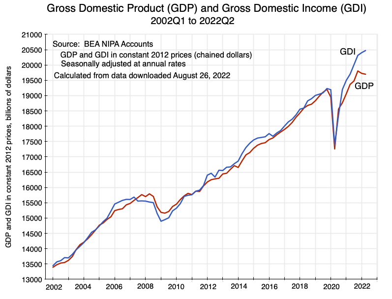
As seen in the chart at the top of this post, these two measures of GDP, while generally moving together over time, have diverged significantly from each other since late 2020.  And in the first half of 2022, GDI continued to grow while GDP fell.  The reasons for this divergence are not clear, but I am sure economists at the BEA are ardently trying to figure this out now.

At this point we do not know what the answer is.  It might well simply be a consequence of the estimates still being recent, and might go away as further data become available to yield better estimates.  But that difference between the two estimates illustrates well why one should not simplistically assert that two quarters of real GDP decline signals a recession underway.

This post will thus first look at the recent data, focusing on what the GDP and GDI concepts mean, why they should be identical (and indeed, for this reason serve as a useful check on each other in the estimates), and what might have caused the recent divergence.  The post will then look at the process followed in the US for designating periods of economic recession and expansion, where for historical reasons the process is overseen not by the government, but rather by a nonpartisan organization called the National Bureau of Economic Research (NBER).  It will conclude with a brief discussion of the prospects for 2023.  While it is doubtful that the economy in the first half of 2022 will ever be designated as being in a recession, the prospects of a recession in 2023, or even later in 2022, are substantial.

B.  Gross Domestic Product and Gross Domestic Income

Gross Domestic Product (GDP) is a measure of production – how much the economy is producing.  But while it is a measure of production, the primary way estimates are made of how much was produced, as well as the way most people think of GDP, is not by how much is produced but by how much is used.  That is, everyone who has taken an Econ 101 macro course will know that GDP will equal the sum of Private Consumption, Private Investment, Government Consumption and Investment Spending (often combined as simply Government Spending – but excluding spending on transfers to households such as for Social Security), and Net Foreign Trade (Exports less Imports).

Why should that sum of expenditures equal production?  The trick (as discussed in this earlier post on this blog) is that investment includes investment in any net buildup of inventories.  That is, changes in net inventories in a period will balance out any difference between what was produced and what was sold.

This is then a convenient way to estimate GDP.  But one should keep in mind that GDP is a measure of production, and that there are other ways to measure that which should yield the same result.  One is to approach it via incomes, as whatever is produced and sold is then someone’s income (when one includes the value of any net inventory accumulation).  Those incomes accrue as someone’s wages (including all forms of labor compensation) or as profits (net operating surplus more formally).  The BEA can assemble available data on wages and profits in the economy, and the sum should in principle be the same as GDP (with adjustments for indirect taxes such as sales taxes and including whatever was set aside in depreciation allowances).  (For those interested in the detailed breakdown, see Table 1.10 in the BEA NIPA Interactive Tables.)  For clarity, the BEA labels this income-based estimate of what should sum also to GDP as Gross Domestic Income, or GDI.

A third approach to estimating GDP is to estimate directly what production was in each sector of the economy.  The BEA does this as well, but one needs to take into account that the net contribution to production in the economy as a whole is not the gross output of any given sector, but that gross output less the value of whatever inputs it purchased from other sectors of the economy.  This is so that one does not double-count what is being produced.  That is, in each sector one estimates what economists call “value-added” – the value of what was produced less the value of the material inputs purchased to make that product.  The sum of this value-added across all sectors should once again be GDP.  The BEA refers to these estimates of value-added by sector as “GDP by Industry”.

The three measures should in principle yield the same figures for overall GDP.  But while in practice generally close, they don’t exactly match as they are all estimates based on data, and the data come from different sources.  Furthermore, that data is subject to revision as more complete information becomes available, so even though initial estimates may differ by some amount, the degree of those differences generally falls over time as better estimates become possible.

Why then does the public discussion generally focus on the expenditure-based estimate of GDP?  One simple reason is that it is always the first one that is published.  The BEA issues this initial estimate of GDP (its “advance estimate”) just one month after the end of the calendar quarter.  This estimate is eagerly awaited both by policymakers and the general public, and receives a good deal of attention in the news media.

The BEA only releases its first estimate of the income-based estimate of GDP (i.e. GDI) a month later, along with its second estimate of the expenditure-based approach to estimating GDP.  Since it comes later, and possibly also because it is less well known, less attention is given by the public (and consequently in the news media) to this income-based estimate of GDP.  But the quarter-to-quarter changes in GDI can differ significantly from the quarter-to-quarter changes in the expenditure-based estimate of GDP.  For example, in the estimates released on August 25, the revised (“second estimate”) for expenditure-based GDP was of a fall of 0.6% in real terms (at an annual rate and seasonally adjusted).  However, the initial estimate of the income-based estimate of GDP (i.e. of GDI) was that GDP grew by 1.4%.  This will be discussed further below.

The initial estimates using the third approach to estimating GDP (i.e. value-added by sector) are then only made available a month after that, i.e. along with the third estimate of the expenditure-based estimate of GDP and the second estimate of the income-based estimate of GDP (i.e. GDI).  These estimates receive even less attention.  The BEA has also been publishing them along with the monthly GDP reports only recently – starting in September 2020 for the second quarter of 2020 GDP figures.  They released them separately before with some further lag, and the underlying data series themselves are only available (in a consistent series based on the current methodology used) from 2005 on a quarterly basis and from 1997 on an annual basis.

Furthermore, while this third approach to estimating GDP could yield an additional check on the GDP estimates, in practice the BEA does not do this.  I am not sure precisely why, but in its methodology for estimating these GDP by Industry figures, it scales the estimates so that the sum matches the expenditure-based estimate of GDP for the period.  The BEA may feel that the underlying data for the GDP by Industry estimates are not sufficiently good to provide an independent estimate of GDP, or it might be concerned that a third but different estimate for GDP might cause confusion in the public.

It is thus not surprising that most attention is paid to the expenditure-based estimates of GDP.  They are available first, and thus they provide the figures that first indicate whether GDP is rising or falling.  But there is also a more fundamental reason why they deserve such attention.  As we have known since Keynes, the primary driver of GDP in the near term is what is happening to the various components of demand for GDP, i.e. the expenditure-based components of GDP.  Production (within the bounds of productive capacity) will respond to those demands, and in particular production will fall when the sum of those demands (what economists call “aggregate demand”) falls.  This might be in response to some financial crisis (with chaos in the financial markets leading to less investment), or to the Fed raising interest rates with the deliberate intention of reducing demand (with the higher interest rates leading to less investment), or due to cuts in government spending (possibly due to politics, such as when the Republican-controlled Congress elected in 2010 forced through government expenditure cuts in the subsequent years, thus slowing the recovery from the 2008/09 financial and economic crash while blaming this on Obama).  Similarly, spurs to growth will be found in what is happening to the various expenditure components of GDP.

The interest in this estimate of expenditure-based GDP is thus well-founded.  But one needs to keep in mind that the figures are still estimates, and are imperfect as the data are imperfect.  An independent check on this, such as from the independent estimate of GDP based on estimated incomes (i.e. GDI), is thus of interest.  Henceforward, for simplicity I will generally refer to the expenditure-based estimate of GDP as simply “GDP”, and the income-based estimate as simply “GDI” (the same terms the BEA uses).

The two estimates (GDP and GDI) generally move quite closely together.  This can be seen in the chart at the top of this post.  Note that while the figures here are shown in real terms, the price deflator used for both GDP and GDI is the same.  The reason is that while price indices can be calculated for the goods and services that make up the expenditure-based estimate of GDP, one cannot define such price indices for the wages and profits that make up the income-based GDI. Thus to deflate the GDI estimate to real terms, the BEA uses the same price deflator as it has estimated for GDP.  This is convenient for the interpretation of the figures as well, as any deviation of one from the other cannot then be attributed in some way to two different price deflators being used.  There is only one.

[Technical Note:  The figures are of GDP and GDI each quarter, but they are shown at annual rates from seasonally adjusted figures.  The price indices used are what are called “chain-weighted dollars”, with 2012 as the base year.  One may recall from an Econ 101 class that a Laspeyres price index calculates the index based on the weights of the underlying items in overall expenditures in the base year, and a Paasche price index calculates the index based on the weights of the underlying items in overall expenditures in the final year.  A chain-weighted index calculates the index based on weights that change period by period based on expenditures on the items in each of the periods.]

The estimates of GDI have generally been above the estimate of GDP in recent years – and especially so since late 2020.  That has not always been the case.  One can see in the chart at the top of this post that estimated GDI was below estimated GDP between mid-2007 and the start of 2011.  But broadly they move together, as one should expect and as can be seen in a chart of the data going back to 1947 (when quarterly estimates of GDP and GDI began):

There is, of course, a scale effect over such a long period, as real GDP has grown by a factor of ten between 1947 and 2022.  The difference between GDP and GDI will not then be so apparent in the earlier years, and it is more meaningful to look at the difference between the two estimates as a share of GDP in that year:

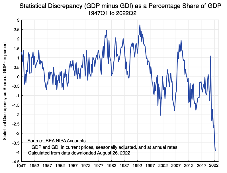
The BEA assigns a label to the difference between GDP and GDI:  they call it simply the “Statistical Discrepancy”.  That difference as a share of GDP was quite small and generally within a range of +/- 1% of GDP between 1947 and the late 1970s, and more often positive than negative (i.e. estimated GDP above estimated GDI).  It then moved between greater extremes, but remained generally positive, from the early 1980s to around 1997.  The volatility then continued, but since 1997 the Statistical Discrepancy was more often negative than positive (estimated GDP less than estimated GDI).

Since the fourth quarter of 2020 it has, however, turned more sharply negative than it has ever been before.  Why?  No one really knows, although there is some speculation (and I am sure work underway at the BEA to try to figure this out).  A higher GDI than GDP implies that estimated incomes are higher than what the expenditure-based estimates would imply.  It is possible that some of these incomes are becoming more difficult to estimate.  For example, there are conceptual issues in how properly to account for compensation being paid by transfers of assets – such as happens with stock options – and the BEA data sources may not be good at estimating these.  Individuals may treat these as part of their compensation (as they should), but in the company accounts they may be treated as a transfer of assets (the stock options) that may not then be properly reflected in recorded profits (at least from the viewpoint of the National Income Accounts).

It is also possible that the sharp increase in the Statistical Discrepancy in the last couple of years may in part go away as more complete data becomes available and new and better estimates for GDP and GDI are worked out.  But at this point we just do not know.

Due to these differences in the estimates, many of the more careful economists working with the GDP figures use not solely the GDP estimate nor solely the GDI estimate, but rather the simple average of the two.  By weighting them equally in this simple average, the implication is that the uncertainty on each is similar.  The BEA itself provides this simple average in its monthly releases of the GDP estimates (although with the item blank in the first release of each quarter when only the expenditure-based GDP estimate is available).  But these figures on the average of GDP and GDI do not receive much attention from many.

Focusing in on the last few years:

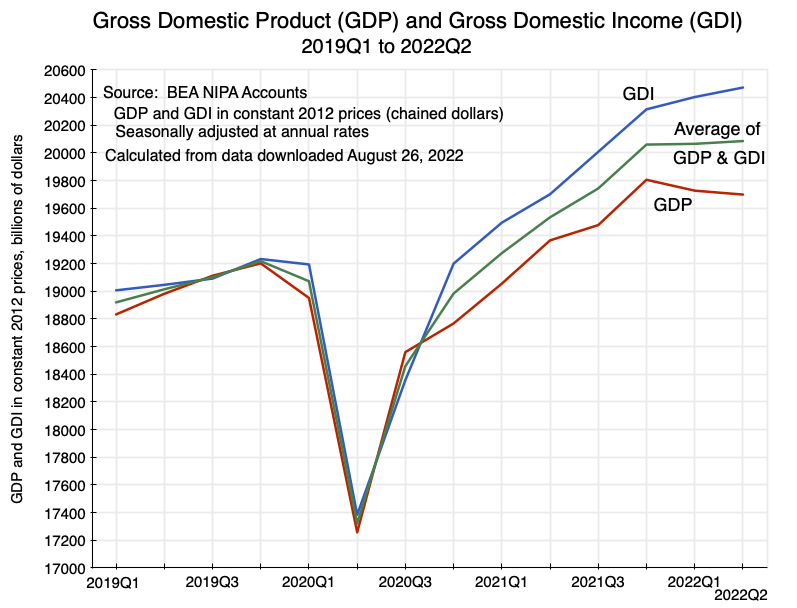
The chart is as before, but now shows also the simple average of the GDP and GDI estimates.  The path of GDP as estimated by the GDI figures has been substantially above the path as estimated by the expenditure-based GDP figures since the fourth quarter of 2020.  And in the first half of 2022, GDI has continued to grow (although at a slower pace than before) while GDP as measured by expenditures fell.  Neither of the changes are large.  And the simple average of the two comes out as almost flat, but positive (with growth of 0.1% in the first quarter of 2022 and 0.4% in the second quarter – in the estimates as currently published).

Thus by this measure of GDP, the economy has continued to grow in these most recent estimates in the first half of 2022, although at only a slow rate.  This could well change with the revisions to come as more complete data become available, but for now they show positive growth in each of the quarters.

C.  Designating and Dating Recessions

The commonly accepted designation of whether the US economy is in a recession or not is not made by a government agency, nor is it based on some set of specific criteria (such as that GDP fell for two consecutive calendar quarters).  Rather, for historical reasons the designation is made through a private, nonprofit and nonpartisan, organization that supports economic research in the US called the National Bureau of Economic Research (NBER).

The NBER was founded in 1920, on the initiative largely of two individuals – one an executive at AT&T and the other a socialist labor organizer who had a Ph.D. in Economics from Columbia.  While very different in their views on what to do about unemployment, both recognized that the data available at the time were insufficient for an adequate understanding of the conditions.  They founded the NBER with the intention for it to support teams that could produce such data – more than what could be done by individual academics.  They deliberately kept it nonpartisan, where the NBER itself would not produce specific policy recommendations, and were able to obtain funding from a range of sources, including from some of the larger corporations of the time, from certain foundations, and from other private donations.

The NBER’s first director of research was Wesley Clair Mitchell, then a professor at Columbia and an expert on business cycle research.  He assembled a team that produced what was then the best data of the time on business-cycle fluctuations in the US.  This research was published and proved influential.  As part of it, as well as in continued such work later sponsored by the NBER, the researchers would determine, to the best the data they could assemble would allow, the periods when the US economy was expanding and when it was contracting.  Periods of contraction were labeled recessions.

The US Department of Commerce started to produce more systematic data on the state of the economy in the 1930s, due in part to the Great Depression then underway.  They worked out the basic GDP concepts we now use and how to measure them in practice given the data they could assemble, with this early work done often with the help of researchers from the NBER.  A particularly prominent such then-young researcher was Simon Kuznets, a student of Wesley Clair Mitchell who then moved to the NBER, and who is often credited with developing the original concepts for GDP (and who subsequently was granted a Nobel Prize in Economics for this work).

The Department of Commerce (now through its Bureau of Economic Analysis) has since produced the official GDP accounts for the US.  In 1961, a decision was made that rather than have this government agency make a determination on whether the economy was in a “recession” (defined in some way) or not, they would instead simply reference the determinations made at the NBER.

These determinations of the NBER were originally made as a by-product of the research it sponsored on business cycles in the US.  In 1978, the NBER decided to formalize the process and make it independent of specific research projects by appointing a committee of academic economists to make such designations.  The committee members represented a range of views but all members had a focus on macro and business cycle issues.  Formally, it was named the NBER Business Cycle Dating Committee.  There are currently eight members of this Committee, and there has been only limited turnover over time.  There have been only seven other individuals who have served on the Committee in the 44 years since its origin, and the chair (Robert Hall), as well one of the current Committee members (Robert Gordon), have served on it since its start.  Robert Hall is a well-respected economist, a professor at Stanford since 1978, and is politically and economically conservative.  He was a supporter of the Reagan tax cuts and has advocated for a flat tax to replace progressive income taxes in the US.

This NBER committee was set up by Martin Feldstein (a professor at Harvard) soon after he became the president of the NBER.  Feldstein was also a well-respected economist as well as open-minded.  He was the Chair of the Council of Economic Advisers in the Reagan White House between 1982 and 1984.  During that time he brought to the Council two bright and capable young economists with recent Ph.Ds. – one to look at domestic policy issues (Larry Summers) and one to focus on foreign trade issues (Paul Krugman).

The NBER Business Cycle Dating Committee meets when members believe they have sufficient data and other information to determine whether the economy had reached a business cycle peak (following which it would be contracting, with this then a recession), or a trough (after which the economy would be expanding, and the recession would be over).  Such determinations have been made by the Committee anywhere between 4 and 21 months after the dates of those business cycle peaks or troughs (as later determined).  They have no deadline for this, but meet when they believe they may have sufficient data to draw a conclusion.  Indeed, sometimes they have met and then deferred a decision, as they felt that upon review they did not yet have sufficient information to make a decision at that point in time (see this news release for one example).

Keep in mind that an economy in recession is one where economic activity is contracting.  It is not defined as a period where economic activity might be considered “low” in some sense, such as below some previous peak.  Thus unemployment will in general still be relatively high at the point where the economy has started to expand again and has thus emerged from the recession.  This may be confusing to some, as economic conditions “feel” (and in fact are) very similar to how they were the month before a trough was reached.  Indeed, it is common that the unemployment rate will still be growing for a period after that trough even though the economic recession (as defined here) is over.  For example, the NBER Committee determined that the 2007/2009 contraction (and thus recession) ended in June 2009.  At that point, the unemployment rate had hit 9.5% – higher than at any point since Reagan (when unemployment peaked at 10.8%).  But the unemployment rate continued to rise after June 2009, peaking at 10.0% in October 2009.

How then is a “recession” defined?  The NBER Committee defines it as:

“a significant decline in economic activity that is spread across the economy and that lasts more than a few months. The committee’s view is that while each of the three criteria—depth, diffusion, and duration—needs to be met individually to some degree, extreme conditions revealed by one criterion may partially offset weaker indications from another.”

Note that it must be what the Committee determines to be a “significant” decline, spread across much of the economy and not simply concentrated in a few sectors, as well as a decline that lasts for a substantial period (normally more than just a few months).  But no specific minimum values are specified for any of these factors.

The Committee also dates the recession (i.e. the dates of the peak and the trough in economic activity) to a specific month.  For this reason alone, the GDP data will not suffice.  It is only available quarterly.  Rather, the Committee has explained that it pays particular attention to the following data series (from the BEA, the Bureau of Labor Statistics, and other sources), which are made available and published monthly:

Real personal income less transfers;

Real personal consumption expenditures;

Employment (both nonfarm payrolls from the Survey of Establishments and employment as reported in the Current Population Survey of households);

Real manufacturing and wholesale/retail trade sales;

Index of industrial production.

But while the Committee has explicitly noted it pays attention in particular to these data series, they can and will look at whatever they feel may be relevant to their decision.

Once they determine the month in which the economy reached a peak or a trough, they will also report on which calendar quarter they believe the economy reached its peak or trough.  This is normally, but not always, the calendar quarter of the respective peak or trough of the months marking a recession, but not always.  Sometimes it might be the quarter before, or the quarter after.  For example, in the short but extremely sharp downturn in the spring of 2020 due to the lockdowns required to deal with Covid, the date marking the start of the recession (when the economy had reached its peak) was February 2020 and the trough was set as April 2020.  But the peak quarter was determined to be the fourth quarter of 2019, not the first quarter of 2020.

It also should be noted that for these determinations of the quarters where the economy had reached its peak or trough, the Committee does not focus on the expenditure-based estimate of GDP, but rather on the simple average of this GDP and GDI.  And as noted above, by this measure GDP rose in the first half of 2022 (according to the current estimates).

Could the Committee get this dating wrong?  Certainly – they are only human, and judgment is required in making these decisions.  Others can and sometimes do disagree, as one would expect in any science.  But the Committee has been careful, makes its decisions only when they believe sufficient time has passed to allow them to make a decision, and the members of the Committee represent a range of perspectives.  And while they do not say so explicitly on the NBER website where they explain their work, I strongly suspect that the Committee operates by consensus, and that if there is not a consensus when some such meeting has been called, they defer their decision until more complete data allows a consensus to be reached.

For this reason, the dates set by the NBER Committee for the beginning and the end of a recession are generally accepted as soundly based.

D.  Conclusion and the Prospects for 2023

Was the economy in a recession in the first half of 2022, as a number of  commentators have asserted?  (See, for example, this report on Fox Business, that asserted the US was in what they called a “technical recession” in the first half of 2022, or these unsurprising statements from Republican Senators Rick Scott of Florida and Rob Portman of Ohio.)

Formally, the NBER Committee has not met on this, so no such determination has yet been made.  But more fundamentally, based on the criteria the Committee uses it is highly doubtful that it will at some point decide the economy was in a recession in the first half of 2022.  The job market as well as other measures have been extremely strong.  Furthermore, even the GDP measure has been misinterpreted in the media as the Committee pays more attention to the average of the estimates for the expenditure-based GDP and the income-based GDI rather than just the former.  By this measure, the economy in fact grew in the first half of 2022 – although not by much and where future revisions in the data might change this.  But even if future data should indicate there was in fact a decline, it would certainly not be by much.

I should hasten to add that this does not mean the economy might not soon be in a recession.  Personally, I believe there is a significant possibility that the economy will be in a recession in 2023, possibly starting later in 2022.  Government spending is coming down sharply from the giant packages passed under Trump in 2020 and then continued under Biden in 2021 to provide relief from the Covid crisis; households are now spending savings that some had accumulated during the pandemic period; and the Fed is raising interest rates with the deliberate intent to slow the economy in order to reduce inflation.  I will expand on each of these in turn.

Using data from the Congressional Budget Office, total federal government spending rose by $2.1 trillion dollars in FY2020 under Trump, an increase of close to 50% from the $4.4 trillion spent in FY2019.  It rose from 21.0% of GDP in FY2019 to 31.3% of GDP in FY2020.  That was gigantic and unprecedented in the US other than during World War II.  It then stayed at roughly that level in FY2021, the first year under Biden (or rather two-thirds of a year as Biden was inaugurated on January 20 and the fiscal year starts on October 1).  In FY2021 federal government spending in fact fell as a share of GDP to 30.5% while rising in dollar value by $269 billion.  But in FY2022 it has now been reduced under Biden by $1.0 trillion – falling as a share of GDP by 7 percentage points to 23.5% of GDP.  There has not been such a fall in government spending since 1947 (as a share of GDP).

In terms of the federal government fiscal deficit, the deficit was at 4.7% of GDP in FY2019 (already substantially higher under Trump than the 2.4% of GDP it was in FY2015, as Trump increased spending while cutting taxes – mostly on the rich and on corporations).  The deficit then jumped to an unprecedented level (other than during World War II) of 15.0% of GDP in FY2020, before falling to 12.4% of GDP in FY2021 under Biden and an expected 3.9% of GDP in FY2022.  Note that this deficit in FY2022 is well less than the 4.7% of GDP in FY2019 under Trump before the Covid crisis.

This sharp cutback in federal government spending under Biden (not the story normally told by Republican politicians) would in itself be deflationary.  It has not been, however, as households as well as businesses are now spending balances many had saved and built up in 2020 and continuing into 2021.  These saving balances were built up from what they received under the various government support programs as well as due to other Covid-related programs (such as the option to suspend payments on certain debts), while spending was kept down (one did not go out to eat at restaurants as often, if at all, for example).  Note this was not the case for everyone.  Many households could only continue to barely get by – spending what they received.  But for other households, the programs led them to increase their savings balances.

The constraints on spending lifted during the course of 2021, and as accumulated savings were spent there was greater demand for goods than supply.  Prices were bid up despite the sharp cutback in government spending in FY2022.  Amplified also as a consequence of the Russian invasion of Ukraine in February 2022 that led to jumps in the prices of foods and fuels, the year-on-year increase in the CPI hit 9.1% in June 2022, before falling some to a still high 8.5% in July 2022.

The jump in the CPI – which started in mid-2021 – has led the Fed to raise interest rates.  Their aim is that the higher interest cost will lead to lower investment, which will reduce aggregate demand.  It hopes to do this without tipping the economy into a recession, but coupled with the sharp cuts in federal government spending and depletion of the excess savings that had built up during the pandemic, there is a significant danger that the Fed will not succeed in this.

It is always tricky, as interest rates are a blunt instrument for moving the economy.  Also, interest rates affect demand only with some lag that is hard to predict.  Finally, if a sharper than desired downturn does appear imminent and some boost in federal government spending becomes warranted to offset this, a Congress controlled by Republicans following the November elections would almost certainly block this.  As discussed above, one saw such dynamics during the Obama presidency following the election of a Republican-controlled Congress in November 2010.  They forced through government spending cuts in the subsequent years, despite the still weak economy following the 2008/09 collapse – the first time there were such cuts in government spending (since at least the 1970s) when unemployment was still high following a recession.  This slowed the pace of the recovery.

There could very well be a repeat of that mistake in 2023.  A recession cannot be ruled out.