Contribution to GDP Growth of the Change in Inventories: Econ 101

An update to this post, looking at the issue from a different perspective, is available here.

This is the first post in a series that I will label “Econ 101”.  Their purpose will be to explain some economic concept that might generally not be clear to many, yet often appears (and often incorrectly) in news reports or other items that readers of this blog might see.  This first Econ 101 post is on how changes in private inventories enter into the National Income and Product (GDP) accounts, where there is often confusion on the contribution of rising or falling inventories to the growth of GDP.

In the most recent (December 22) release by the government of the GDP accounts in the third quarter of 2011, growth in overall GDP was an estimated (and disappointing) 1.8%. But many news reports stated that private inventories fell, and that had these inventories not changed, GDP growth would have been 1.4% points higher, or a more respectable 3.2%.  Yet when one looks at the underlying GDP figures issued by the BEA (the Bureau of Economic Analysis, US Department of Commerce), one sees that the change in private inventories was essentially zero (and in fact was slightly positive).  If inventories did not fall, why did many commentators state that a fall in inventories reduced GDP growth in the quarter?

The confusion arises because while the GDP (Gross Domestic Product) accounts measure the flow of production (how much was produced during some period of time), and the flow of how much was then sold (e.g. for consumption or investment), inventories are a stock, and it is the change in the stock of inventories that enters into the GDP accounts.  GDP is the flow of goods and services produced in the economy, and these goods and services are then sold for various purposes, including private consumption, private fixed investment, government consumption and investment, and exports, with imports also a supply of goods that can be sold.  But goods produced in some period will not necessarily match goods sold in that same period.  The difference is accounted for by either a rise or a fall in inventories.  Hence the change in the stock of inventories, when added to final sales (with imports entering as a negative), will equal total goods and services produced, which is GDP.

From one period to the next, we are normally interested in how much GDP rose or fell in that period compared to the previous one.  And we are interested in seeing how much of that growth in GDP will match up with and can be accounted for by growth of consumption, investment, and other elements of final sales.  These demand components are important, particularly in the economy as it is now.  With high unemployment and production well less than capacity, production of goods and services is driven by the demand for them.  Hence one is looking at the change in consumption or fixed investment or government expenditures from one period to the next.  And as the balancing item between GDP production and final sales, one would now be looking at the change in the change in inventories.

The term “the change in the change in inventories”  is a mouthful, and not often seen in news reports (indeed, I have never seen it used).  But that is what then leads to the confusion.  In the third quarter of 2011 (in the estimates released by the BEA on December 22), the change in private inventories was essentially zero, as noted above.  But there had been some positive growth in private inventories in the second quarter of 2011. Hence, the change in the change in inventories, going from something positive to essentially zero, was negative.  That is, if inventories had continued to increase in the third quarter of 2011 as much as they had in the second quarter, GDP growth would not have been 1.8% but rather would have been 3.2%.  The change in the change in inventories meant GDP growth was 1.4% points less than what it otherwise would have been.

The point can perhaps best be illustrated by some simple numerical examples.  Suppose for some fictitious economy, that GDP (the production of goods and services) is initially 1000 (in, say, billions of dollars), while the total of final sales (for consumption, fixed investment, and so on) is 950.  With production of 1000 and sales of 950, inventories will increase by 50.  Assume the stock of inventories at the start of the period is 500, so the stock will total 550 (50 more) by the end of the period.  The figures are as in this table:

Period 1 Period 2 Change % Change
GDP 1000 1050 +50 5%
  Change in Inventories  50  80 +30 3.0% points
  Final Sales 950 970 +20 2.0% points
Stock of Inventories:
    Start 500 550
    End 550 630
In the second period, suppose that production (GDP) increases by 50, or 5%, to 1050, while final sales only grow by 20, to 970.  The difference between production and sales must accumulate in inventories, so the change in inventories will now be 80.  Therefore, the change in the change in inventories will be 30 ( =80-50), and the contributions to the 5% growth in GDP will be 2.0% points from the change in final sales, and 3.0% points from the change in the change in inventories.  It is also worth noting that the stock of inventories has now grown to 630 by the end of the second period, which is substantially higher as a share of GDP or of final sales than it was at the start of period 1.  Hence, there is reason to assume that producers will likely scale back production (GDP) in the near future as long as final sales growth remains so sluggish, as there is likely little reason to accumulate even more unsold inventories on the shelves.
.
The second example will illustrate the case where inventories continue to rise, but at a slower pace than in the first period:
Period 1 Period 2 Change % Change
GDP 1000 990 -10 -1%
  Change in Inventories  50  20 -30 -3.0% points
  Final Sales 950 970 +20 +2.0% points
Stock of Inventories:
    Start 500 550
    End 550 570
In this example, final sales still grows by 20 to 970.  But producers here have scaled back production to just 990, or 1% below what it had been, with inventories now growing by just 20 rather than the 80 of the first example.  The change in inventories is still positive (at +20), but the change in the change in inventories is now negative, at -30.  The contributions to the -1% growth in GDP growth is made up of +2.0% points from final sales, and -3.0% points from the change in the change in private inventories.
As a final example, we will look at a case where the change in private inventories is negative.
Period 1 Period 2 Change % Change
GDP 1000 1050 +50 5%
  Change in Inventories -50 -20 +30 +3.0% points
  Final Sales 1050 1070 +20 +2.0% points
Stock of Inventories:
    Start 500 450
    End 450 430
Final sales once again grows by 20, although now from 1050 to 1070.  Sales is greater than production in each period, and inventories are drawn down by 50 in the first period and by 20 in the second period.  But while the change in inventories is negative in each period, that change is less negative in the second period than it is in the first.  That is, the change in the change in inventories is a positive 30, and this accounts for 3.0% points of the 5% growth in GDP.  It is also valuable to note that with inventories falling in each period, the total stock of inventories by the end of the second period is getting fairly low, so it is reasonable to expect that producers will aim to replenish inventories in future periods, with this then acting as a spur to growth.
.
Such swings in inventories are often important when economic growth is turning around, as at the start of a recovery from a downturn, or at the start of a downturn following a boom.  An example is seen at the end of the most recent recession, in the middle of 2009. The economy was in a state of collapse in 2008, the last year of the Bush Administration, and this fall carried over into the first half of 2009.  This downturn was then halted and reversed as a result of the policies implemented at the start of the Obama Administration. GDP was falling at a huge 8.9% annual rate in the last quarter of 2008, and at a still very high 6.7% rate in the first quarter of 2009.  Growth was then still negative, but at only a 0.7% rate, in the second quarter of 2009, and then started to grow at a 1.7% rate in the third quarter, and at a 3.8% rate in the fourth quarter.
.
The change in private inventories was negative in each quarter throughout this period. Specifically, private inventories fell by $200.5 billion in the second quarter of 2009, fell again by $197.1 billion in the third quarter, and fell again by a further $66.1 billion in the fourth quarter.  But the change in the change in private inventories was positive in the third and fourth quarters (while negative in each, they were becoming less negative), and this then accounted for a positive 0.2% points of the 1.7% growth in GDP in the third quarter, and a strong 3.9% points of the 3.8% growth in the fourth quarter (when final sales in fact declined slightly, accounting for a -0.1% contribution to growth in that period).
.
To summarize:  As everyone knows from their first Econ 101 class in Macroeconomics, GDP is equal to Consumption + Investment + Government Spending + Net Exports (Exports minus Imports), where total Investment is equal to Fixed Investment plus the Change in Inventories.  The change in GDP will therefore equal the change in Consumption + the change in Investment + the change in Government Spending + the change in Net Exports, where the change in Investment will equal the change in Fixed Investment plus the change in the Change in Inventories.
.

New Home Sales Remain Abysmal, But The Potential Should Be Recognized

New home sale figures for October, recently released, remain abysmally low at just 307,000 sales at an annual rate.  They have fluctuated within only a narrow range over the past year, with no clear trend and no signs to be encouraged by.  What is more interesting is the longer term context.

New home sales in the US fluctuate a good deal, but around a rising trend of 1.0% a year (calculated from a regression over the 1980 to 2010 data).  They reached a fairly stable level of approximately 900,000 housing units a year between 1998 and 2001.  But there was then a bubble between 2002 and 2006, reaching a peak of almost 1,300,000 in 2005, and then crashing to a bit over 300,000 in 2010 and 2011, where it now seems to have leveled off.

Only 300,000 new home sales a year is abysmal and a major drag on the economy.  It is only one-third of the 900,000 level of the early part of the last decade, and less than one-quarter of the levels reached in the bubble years.  But it should also be noted that people need homes, and that that need grows over time due to population growth.  The trend 1.0% growth found in the data is consistent with this.  And with new home construction now far below trend, it will be a significant spur to the economy if and when housing construction recovers.  Brad DeLong has made a similar point in his blog a number of times.  Here is one such post.

Keeping things simple and conservative, let’s assume that new home sales will, for the purposes here and over periods of time, on average equal the number of new homes constructed.  All are eventually sold, with very few exceptions.  And while there are figures available for new housing starts, these are consistently higher than sales for reasons that are not clear, but may reflect homes never completed.  Using the 900,000 units sold a year between 1998 and 2001 as a reasonable norm, and for simplicity not even allow for a rising trend in this figure, one can calculate the excess over the bubble years 2002 to 2006 (the area in blue in the graph) and then the shortfall that has developed over 2007 to 2011 and continues (the area in red).  Based on the figures underlying the graph, the excess during the bubble was 1.1 million units, while the shortfall in the subsequent bust through 2011 was 2.2 million units.  There is therefore now a net shortfall in housing supply of 1.1 million, as the excess over 2002 to 2006 has been more than worked off.  And as long as new home sales and construction remain at only 300,000 a year, that shortfall (relative to a 900,000 per year norm) will be growing by 600,000 housing units a year.

This suggests that a major pent-up demand for homes has built up.  It has not been resolved due to continued problems in the housing market and especially in the housing finance market, with many mortgages underwater and hence do not move, mortgages that remain hard to get by potential new buyers, an overhang of houses not sold, and a foreclosure process that has not worked well.  The market remains close to frozen.

But if these housing market problems could be resolved, so that construction could revert to its previous norms, the stimulus to the economy would be huge.  Assuming simply a return to construction of 900,000 units a year (and hence ignoring what would likely be an overshooting of this for a few years to make up for the net shortfall of recent years), implies construction of an additional 600,000 units a year.  At the average new home price of $221,800 in 2010, the aggregate value of such homes would be $133 billion per year.  This is just short of 1% of GDP.  Most of this would add to GDP as there is some, but only limited, “leakage” through some inputs that are imported (housing lumber, fuel for trucks, etc.).

But there will also be indirect multiplier effects, especially in the current depressed economy.  A reasonable estimate of the multiplier on housing construction would be 2 to 3.  A return of new home construction to previous levels would therefore add 2 to 3% of GDP. With actual GDP currently about 5% below potential GDP (estimate for end 2011 by the Congressional Budget Office, page 12), such an addition from housing construction would bring the economy about half-way back to where it needs to be.  But this will not happen until the market for homes and for home mortgage financing begins to function reasonably well.

GDP Growth in the Recovery Remains Slow, But Policies Are Not Holding Back Business Investment

GDP growth in the economic recovery from the 2008 collapse remains weak.  The recently released GDP figures for the second quarter of 2011 (second revision, from the Bureau of Economic Analysis of the Department of Commerce), revises downward the growth estimate to 2.0% from the previous estimate of 2.5% (all figures are quarter on quarter growth, seasonally adjusted at annual rates).  While still positive, and better than earlier in the year, such growth is insufficient to bring down the still high unemployment to a significant degree.

Four points:

  1. The overall GDP growth rate would have been 1.55% points higher (i.e. a more decent 3 1/2%) if the change in private inventories had remained the same as it had been in the second quarter of 2011.  Over time, the contribution to GDP growth from inventory accumulation is on average close to zero, so one would expect that over the next couple of quarters this will switch back to positive from negative to balance out desired inventories.  Note that the contribution to the growth in GDP in any period is the change in the change in private inventories.  Private inventories did not fall in the third quarter of 2011:  they merely failed to grow as fast as they had in the second quarter.  I will try to prepare a methodology note discussing this arithmetic at some point in the future, and post it in the Econ 101 section of this blog.  (Update:  It is now posted here.)
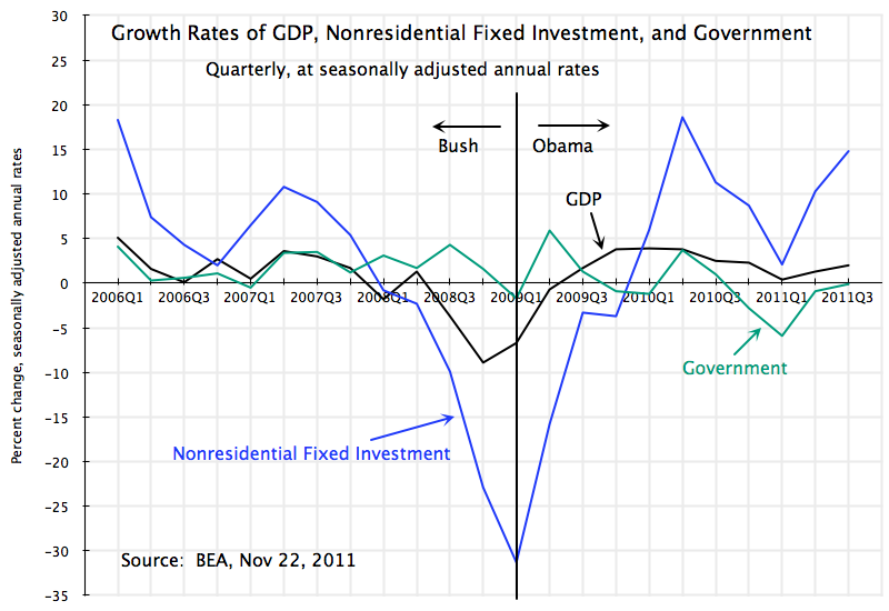
  2. Obama has been strongly criticized by Republicans that his policies have been anti-business, and hence have led business not to invest, with this then resulting in the disappointing growth of GDP.  But the figures do not support this.  Business investment has in fact been quite good, as seen in the figure above, with growth of 15% in the most recent quarter, and generally quite strong growth since the beginning of 2010.  This is especially surprising as capacity utilization (as estimated by the US Fed) is still only 78% of potential capacity (and while never at 100%, this figure will be at around 85% when the economy is close to full capacity utilization).  Business is investing even with the current excess in capacity.
  3. An economic headwind that has been hurting growth, starting in late 2010 and then into 2011, has been the fall in government demand.  This has principally been from cutbacks in state and local governments.  If government demand had simply not been cut, GDP growth would have been about half a percentage point higher than what it was from simply the direct impact of the government cut-backs, and even higher if multiplier effects are included.
  4. And, perhaps stating the obvious, while Obama is now being blamed for the downturn, the critics need to be reminded that the sharp collapse in output came in 2008.  This was then turned around in 2009, after Obama took office, with growth since.  The growth has not been fast enough, and the economy remains well below its potential capacity, but reverting to the previous policies is the last thing one should do.