The Rate of Economic Growth and the Budget Gap: Returning to the Long-Term Average Growth Rate Would Eliminate It

Long Run US GDP per Capita Growth (1870-2088) in logarithms

Larry Summers published an op-ed yesterday (appearing in Reuters, the Financial Times, the Washington Post, and probably elsewhere) in which he makes the important point that the current budget impasse is focussed on the wrong issues.  The discussion, at least as publicly expressed, has focussed on what is seen as needed to deal with the fiscal deficit and the resulting public debt.  Even the Republican attempt to end ObamaCare was ostensibly about cutting the government deficit (even though the CBO concluded that the opposite would happen, as they found that the ObamaCare reforms will reduce the deficit, rather than increase it).

Yet this focus on near term and projected budget deficits is misguided.  As Summers notes, under current policies the public debt to GDP ratio is falling, and is projected to continue to fall into the 2020s.  The recently issued Long-Term CBO budget projections indicate that while the debt ratio would then start to rise (primarily driven by expected higher health care costs), there is a good deal of uncertainty in those projections.

Specifically the CBO figures show that it would not take much, in terms of either higher revenues or lower spending, to keep the public debt to GDP ratio flat.  Higher revenues or lower spending or some combination of the two, of 0.8% of GDP over the next 25 years or 1.7% of GDP over the next 75 years, would suffice.  This is consistent with an earlier post on this blog, which showed that if the Bush tax cuts had not been extended for almost all households, the projected debt to GDP ratio in the CBO numbers would fall rapidly.

But projections of revenues or of spending are highly uncertain.  Projected health care spending has been coming down steadily in recent years, for example, in part due to the slow economy, but also in part as a result of the efficiency gains and cost reductions that the ObamaCare reforms are leading to.  With these lower costs, the CBO has been steadily reducing the projected costs to the government budget from Medicare, Medicaid, and other such health programs.  In the recent CBO report, for example, the projections of government spending on health care programs in the 2030s were reduced by 0.5% of GDP from what the CBO had projected just one year earlier.  Going back further, the CBO projections for government spending on health care in 2035 were over 1% of GDP lower in the projections recently issued than in the projections published in June 2010.

This should not be interpreted as a criticism of CBO.  Their projections are probably the best available.  Rather, the point is that these projections are inherently hard to do, and the uncertainty surrounding them should not be ignored.  Yet the politicians often ignore precisely that.

Furthermore and perhaps most importantly, the projected budget deficits and resulting public debt to GDP ratios depend critically on the rate of growth of the economy.  The CBO uses a fairly detailed and reasonable model to project this (based on projected labor force growth, investment in capital, and productivity growth).  However, it is probably even more difficult to project GDP than to project future spending levels and tax revenues for any given level of future GDP.  But Summers notes the critical sensitivity of the projected future deficits to the projected growth in GDP.  He states “Data from the CBO imply that an increase of just 0.2 percent in annual growth would entirely eliminate the projected long-term budget gap”.

One can calculate from the data made available with the CBO report their projected growth of real per capita GDP.  For 2013 to 2088, it comes to 1.60%  year.  A previous post on this blog noted the remarkable constancy of the rate of growth of real per capita GDP since at least 1870 of 1.9% a year (or 1.87% a year at two digit precision).  That earlier post noted that real per capita GDP in the US, despite large annual variations and even decade long deviations (such as during the Great Depression, and then during World War II), has always returned to a path of 1.87% growth since at least 1870.  That path even did not shift when there were even substantial deviations, such as during the Great Depression.  Rather, the economy always returned to the same, previous, path, and not one shifted up or down.

This is truly remarkable, and no one really knows the reason.  The path can be seen as a trend growth of capacity (based on labor available and capital invested, coupled with the technology of the time), but why this should path should have grown at 1.87% a year in the late 1800s; in the early, mid and late 1900s; and all the way into the 21st century, is not known.

Since we do not know why the economy has always returned to this one path, we need to be careful in looking forward.  Still, it is noteworthy that the CBO projections imply that the economy will now slow, to just 1.60% real per capita GDP growth over the next 75 years.  This CBO path is substantially lower than the path of 1.87% growth that has ruled for the last 140 years in the US.

The graph at the top of this post shows the path of GDP per capita projected by the CBO (which one should note is a year by year projection, which just averages out to 1.60% per year over the full period), along with an extension of the 1.87% path that has ruled since at least the 1870s.   The graph is adapted from my earlier post (although now converted to prices of 2005 whereas the earlier one was in prices of 1990; this does not affect the rates of growth).  It is expressed in logarithms, since in logarithms a constant rate of growth is a straight line.

It is not clear why there should be this deceleration to 1.60% from the 1.87% rate of growth the economy has followed over the last 140 years.  Mechanically, one can ascribe the deceleration to what the CBO assumes for the rate of growth of technological progress.  But projecting growth in technology over a 75 year period is basically impossible, as the CBO notes.

The deceleration over the next 75 years has a very important implication, however.  The CBO found in its sensitivity analysis that a rate of growth that is just 0.2% faster will suffice to close the budgetary gap, even if one does not take any new measures to raise revenues or cut government spending.  Hence a return to the previous historical growth path of 1.87% a year from the 1.60% rate the CBO projects, or a difference of 0.27%, will more than suffice to close the budgetary gap.

The policy implication is that with such sensitivity to the growth in GDP, we should be focussed on measures to raise growth, rather than short term budgetary measures that will act to reduce growth.  The economy has suffered from government austerity since 2010, which has held back growth.  Government has been cutting spending, thus undermining demand in an economy with high unemployment and close to zero interest rates, where more labor is not employed and more is not produced because the resulting products could not then be sold due to the lack of demand.  As an earlier post on this blog noted, if government spending had been allowed to grow simply at the historic average rate (and even more so if it had been allowed to grow as it had under Reagan), the US would by now be back at full employment.

Over the medium term, Summers notes that both conservatives and liberals agree that growth should be raised, and on the types of measures which should help this.  More investment, both public and private, is required rather than less.  Research and development, both public and private, is important.  More effective education is also required.

I would agree with all of these.  But to be honest, since we do not really understand why the economy always returned to the 1.87% growth path over the last 140 years, it would not be correct to say we can be sure such measures will be effective.  However, what we can say with confidence is that measures that hinder the recovery of the economy, as the government spending cuts have been doing, will certainly hurt.

The Recovery From the 2008 Collapse That Could Have Been: The Impact of the Fiscal Cuts

GDP Recovery Path with Govt Growth at Historic Average, 2004Q4 to 2013Q2

A.  Introduction

Previous posts on this blog (including this older one from 2012) have discussed how the sluggish recovery from the 2008 economic collapse could have been avoided if one had allowed government spending to grow as it had during Reagan’s term.  This post will look in more detail at what the resulting path for GDP would have been if government spending had followed the path as it had under Reagan, or even had simply been allowed to grow at its normal historical rate.

The 2008 collapse was of course not caused by fiscal actions, but rather by the bursting of the housing bubble, and its consequent impact both in bankrupting a large share of an overly-leveraged financial system and in causing household consumption to fall as many homeowners struggled to repay mortgages that were now greater than the value of their homes.  Faced with the high unemployment resulting from this, an expansion of government spending would have supported the demand for output and hence for workers to produce that output.  And initially, fiscal spending did indeed grow.  This growth (along with aggressive action by the Fed) did succeed in turning around the steep slide of the economy that Obama faced as he took office.  But since 2009 government spending has been cut back, and as a result the recovery of GDP has been by far the slowest in any cyclical downturn of the last four decades.

This blog post will look at alternative scenarios of what the recovery path of GDP could have been, had government spending not been reduced.  Two primary alternatives will be examined.  In the first, government spending is allowed to grow from the point President Obama took office at a rate equal to its average rate of growth over the period 1981 to 2008.  In the second, government spending is allowed to grow from the onset of the recession (i.e. from the fourth quarter of 2007) at the same rate as it had during the Reagan years, following the downturn that began in the third quarter of 1981.

B.  Government Spending Growth at the Historic Average Rate

In the first scenario, real government spending on goods and services (as measured in the GDP accounts, and inclusive of state and local government as well as federal) is allowed to grow at a rate of 2.24% per year.  This is the average rate of growth for government spending over the 28 years from 1980 to 2008.  This was a modest growth rate, and spanned the presidencies of three Republicans (Reagan and the two Bushes) for 20 of the 28 years, and one Democrat (Clinton) for 8 of the 28 years.  The 2.24% growth rate was substantially below the growth rate of GDP of 3.04% over this same period (note this is for total GDP, not per capita).  As a result, real GDP grew by over 50% more over this period than government spending did.  But this modest pace of government spending growth was substantially more than the absolute fall in government spending during Obama’s term in office.

Note that this path for government spending is not some special rate faster than the historical average, as would normally be called for in a downturn when fiscal stimulus is needed because aggregate demand in the economy is less than what is needed for full employment.  Rather, it is just the historical average rate.  This should be seen as a neutral path, with government spending neither purposely stimulative, nor purposely contractionary.

This path for government spending is shown as the orange line in the following, where the path is superimposed on the graph presented in the earlier blog post of such paths of government spending in each of the downturns the US has faced since the 1970s:

Recessions - Govt Cons + Inv Expenditures Around Peak, 12Q before to 22Q after, with growth at avg historical rate

Maintaining government spending growth at the historical 2.24% rate would have led to government spending well below that seen during the Reagan years (in the recoveries from the July 1981 and January 1980 downturns), roughly where it was in the recoveries from the November 1973 and March 2001 downturns, and well above where it was in the recoveries from the July 1990 downturn (during the Clinton years) and of course the December 2007 downturn (under Obama).  Government spending in the current downturn (the brown curve in the graph) has fallen substantially during the period Obama has been in office.

The graph at the top of this post then shows what the GDP path would have been if government spending would have been allowed to grow at the historic average rate.  The impact will depend on the multiplier.  As was discussed in the earlier post on fiscal multipliers, the multiplier for the US in this period of high unemployment and short-term interest rates of close to zero will be relatively high.  But for the purposes here, we will run scenarios of multipliers of 1.5, of 2.0, and of 2.5.  This will span the range most economists would find reasonable for this period.

The results indicate that had one simply had government spending grow at its historic average rate, the economy would likely now be at or close to potential GDP, which is what GDP would be at full employment.  But because of the fall in government spending since 2009 rather than this increase, current actual GDP is over 6% below potential GDP, and unemployment is high.  (Potential GDP comes from the CBO estimates used in its May 2013 budget projections, but adjusted to reflect the methodological change made by the BEA in July 2013.  Due to these adjustments, including for the GDP deflators used, the potential GDP path is not as “smooth” as one would normally see.  But it will be close.)

Republicans have argued that we cannot, however, afford higher government spending, even if it would lead the economy back to full employment, as it would lead to an even higher public debt to GDP ratio.  But as was discussed in a recent post on this blog on the arithmetic of the debt to GDP ratio, it is not necessarily the case that higher government spending will lead to a higher ratio.  The Republican argument fails to recognize both that GDP will higher (due to the multiplier, and indeed a relatively high multiplier in the current conditions of high unemployment and close to zero short-term interest rates), and that a higher GDP will generate higher tax revenues due to that growth, which will off-set at least in part the impact on the deficit of the higher spending.

The resulting paths for the debt to GDP ratios by fiscal year, using a 30% marginal tax rate for the higher income, would be:

Public Debt to GDP with Govt Growth at Historic Average, FY2009 to FY2013

The impact of the higher government spending is to reduce the debt to GDP ratios over this period.  The higher government spending leads to a higher GDP, and this higher GDP along with the extra tax revenues generated at the higher output means the debt rises by proportionately less.  The ratios fall the most, as one would expect, the higher the multiplier.  If one is truly concerned about the burden of the debt, one should be supportive of fiscal spending in this environment to bring the economy quickly back to full employment.  The debt burden will then be less.

The debt to GDP ratios still rise over these years.  This serves to point out that the assertion made by the Republicans that the public debt to GDP ratio has risen so much during Obama’s term due to explosive spending under Obama is simply nonsense.  The debt to GDP ratios rose not due to higher government spending, but primarily due to the economic collapse and slow recovery, which has decimated tax revenues.  With higher government spending, the debt to GDP ratios would have been lower.

C.  Government Spending Growth at the Rate During the Reagan Years

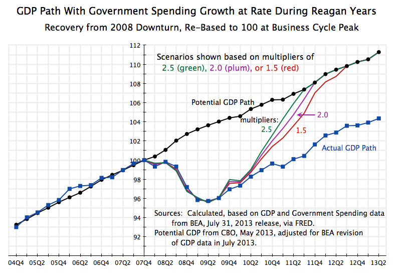
The second set of scenarios examine what the path of GDP would have been had government spending been allowed to grow, following the onset of the downturn in December 2007, at the same pace as it had during the Reagan years following the onset of the July 1981 downturn.  The path followed is shown as the green line in the graph above on government spending around the business cycle peaks.

The resulting recovery in GDP during the current downturn would have been significantly faster:

GDP Recovery Path with Govt Growth at Reagan Rate, 2004Q2 to 2013Q2

If government spending had been allowed to grow under Obama as it had under Reagan, the economy likely would have reached full employment in 2011 (multipliers of 2.5 or 2.0), or at least by the summer of 2012 (multiplier of just 1.5).  That is, the economy would have been at full employment well before the election.

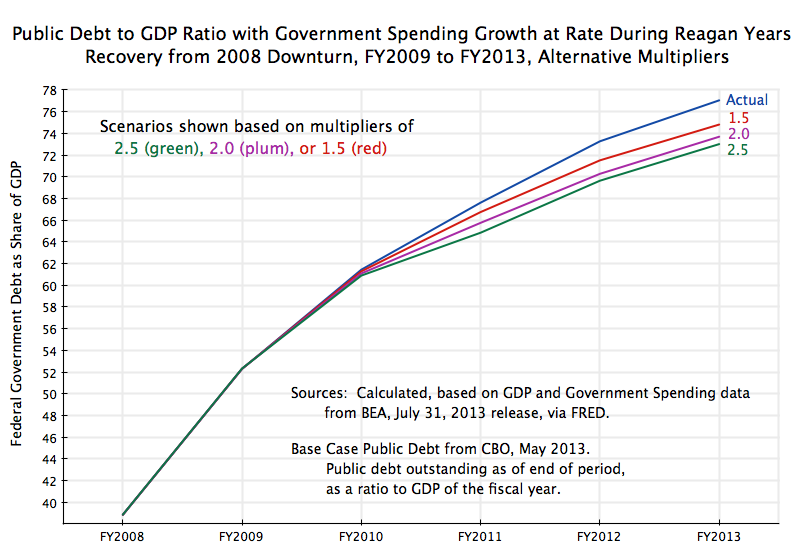
The deb to GDP ratios would also have been less than what they actually were:

Public Debt to GDP with Govt Growth at Reagan Rate, FY2008 to FY2013

Note that for these calculations I assumed that once the economy reached full employment   GDP (potential GDP), that government spending was then scaled back to what was then necessary to maintain full employment, and not over-shoot it.  Hence the curves for the 2.5 and 2.0 multipliers move parallel to each other (and are close to each other) once this ceiling has been reached.

D.  Conclusion

Fiscal spending was not the cause of the 2008 collapse.  Rather, the cause was the bursting of the housing bubble, and the resulting bankruptcy of a large share of the financial system, as well as the resulting reduction in household spending when many homeowners found that their homes were now worth less than their mortgages.

But following an initial increase in government spending, in particular as part of the fiscal stimulus package passed soon after Obama took office, government spending has been cut back.  The scenarios reviewed above indicate that had government spending merely been allowed to grow at its normal historical rate from when Obama took office (i.e. even without the special stimulus package), the US would by now be at or at least close to full employment.  And if government spending had grown as it had during the Reagan years, the economy would likely have reached full employment in 2011.

There is no need to introduce some special factor to explain why GDP is still so far below what it would be at full employment.  There is no need to assume that something such as “business uncertainty” due to Obama, or new and burdensome regulations, have for some reason led to this slow recovery in GDP.  Rather, the sluggish recovery of GDP and hence of employment can be explained fully by the policies that have kept government spending well below the historical norms.

An Increase in Government Spending Can Reduce the Debt to GDP Ratio: Econ 101

Most people realize that it is not the absolute value of the government debt that matters, but rather the ratio of that debt to GDP.  A larger economy can support a larger debt.  But most people will also think instinctively that an increase in government spending will necessarily lead to an increase in the government debt to GDP ratio.  It is not surprising that they should think so.  But it is wrong.

Whether the government debt to GDP ratio will rise or will fall when government spending increases will depend on economic conditions and other structural factors.  In conditions of high unemployment and where the Central Bank has driven the interest rates it can control essentially to zero, such as exist now in the US and Europe, an increase in government spending will increase the demand for goods and services, and hence will increase the demand for labor to produce those goods and services.

Employment and output will then rise. How much they will rise will depend on the multiplier, but as was discussed in a previous Econ 101 post on this site, in conditions of high unemployment and close to zero Central Bank controlled interest rates such as currently exist, the multiplier will be relatively high.  The higher incomes that then follow from the higher employment and output will also then lead to higher tax revenues, as a share of the higher incomes will be paid in taxes.

Hence the addition to the deficit and thus the public debt will be less than simply the increase in government spending, due to the higher tax revenues.  With GDP higher due to the greater demand and with the debt also possibly higher but not by as much, the debt to GDP ratio could fall.  And indeed, under conditions such as currently exist in the US and Europe, the debt ratio will almost certainly fall.

To see this, one can start with a simple numerical example.  Suppose one starts with a GDP equal to 100 units (it could be $100 billion), a public debt of 50 (or 50% of GDP, roughly where it was in the US in 2009), a multiplier equal to 2.0 (a reasonable estimate for the US in recent years), and a marginal tax rate on additional income of 30% (also a reasonable estimate for what it is for US federal government level revenues; it would be higher if one included state and local government revenues).

In these conditions, suppose government spending rises by 1 unit.  With a multiplier of two, GDP will then rise by 2 units.  Tax revenues will then rise by 0.6 units, when the marginal tax rate is 30% on the additional 2 units of GDP.  The government deficit, and hence the public debt, will rise by 0.4 units, equal to the extra 1 unit of government spending less the 0.6 units of additional tax revenue.  The resulting public debt will be 50.4, while GDP will then be 102, and the ratio of 50.4/102 is equal to 0.494.  Hence the debt ratio fell from 50% to 49.4% when government spending rose by 1.  Higher government spending led to a reduction in the debt to GDP ratio.  While the total debt rose, GDP rose by proportionately more, leading to a fall in the debt to GDP ratio.

Further numerical examples will help give a feel to what is going on:

Impact on Debt/GDP Ratio from a One Unit Increase in Government Spending
        Scenario: (a) (b) (c) (d) (e)
GDP: Y 100 100 100 100 100
Public Debt: D 50 70 30 50 50
multiplier: m 2.0 2.0 2.0 0.5 3.5
marginal tax rate: t 0.3 0.3 0.3 0.3 0.3
pre-change D/Y 0.500 0.700 0.300 0.500 0.500
Change in G 1 1 1 1 1
Change in Y 2 2 2 0.5 3.5
Change in D 0.4 0.4 0.4 0.85 -0.05
Resulting D/Y 0.494 0.690 0.298 0.506 0.483

Scenario (a) is the case just discussed.  With an initial public debt ratio of 50%, a multiplier of 2, and a marginal tax rate of 30%, a unit increase in government spending will lead the debt to GDP ratio to fall to 49.4%.  This is robust to different initial debt to GDP ratios:  The debt to GDP ratio will fall with higher government spending with an initial debt ratio of 70% (scenario (b), with the debt ratio where it was in FY2012) or at 30% (scenario (c), almost what the debt ratio had fallen to at the end of the Clinton administration, before the Bush tax cuts).

Under conditions where the economy is close to full employment, so that the multiplier will be relatively small, the debt ratio could rise with the higher government spending.  GDP will not rise by much, if at all, if the economy is already producing at or close to full employment levels.  The denominator in the ratio hence will not rise by much, if at all, while the numerator (the level of debt) will rise by the level of extra government spending, with only limited or no extra tax revenues to offset this since GDP has not increased by much.   Scenario (d) provides an example, with a multiplier of 0.5.  The debt ratio will rise from 50% to 50.6% in this example, when government spending rises by 1.

At the other extreme, a very high multiplier may lead to such a large increase in GDP that the extra tax revenues thus generated are greater than the increase in government spending, leading to an actual decrease in the deficit and hence the debt.  Scenario (e) presents an example, with a multiplier of 3.5.  Debt actually falls from 50 units to 49.95 units, despite the increase in government spending by 1 unit, and the debt to GDP ratio falls from 50% to 48.3%.

One will also get this result if the extra tax revenues generated for a given increase in GDP is sufficiently high.  The above examples assume a marginal tax rate of 30%.  More generally, if the marginal tax rate times the multiplier is greater than one (e.g. 30% times 3.5 = 1.05 in the example above), then the absolute value of the debt will fall with the higher government spending.

It may well be unlikely, however, that the multiplier will be as high as 3.5, even with the current high unemployment in the US and Europe.  Thus it is unlikely that the absolute value of the debt will fall with higher government spending, even in conditions of high unemployment.  But as was discussed above, with a reasonable estimate of the multiplier at around 2, one will see the debt to GDP ratio fall, under conditions such as now exist in the US and Europe.

For those with some mathematical expertise, it is straightforward to derive the specific conditions which will determine whether the debt to GDP ratio will rise or fall with an increase in government spending.  This requires some elementary differential calculus, and I will not go through the derivation here.  But the final result is that the debt to GDP ratio will fall if:

(t + D/Y) – (1/m) > 0

and the debt ratio will fall if the sum on the left is less than zero.  That is, the debt to GDP ratio will fall if the marginal tax rate (t), plus the initial debt to GDP ratio (D/Y), minus the inverse of the multiplier (m), is greater than zero (and will rise if the sum is less than zero). Thus if t=30%, D/Y=50%, and m=2 (so 1/m=0.5), with a sum then of 0.3 + 0.5 – 0.5 = 0.3, which is greater than zero, the debt to GDP ratio will fall.

The material above is straightforward.  There is nothing deep or complex.  It also just examines the immediate impact on the public debt to GDP ratio from an increase in government spending.  For a more elaborate look at the long-term impact, see the paper of Brad DeLong and Larry Summers published in 2012.  They show there that higher government spending will not only spur GDP in the short run under conditions such as exist now, but also that such spending will likely pay for itself in the long run through its long term positive impact on growth.

But this post simply focuses on the short term, and shows that counter to what many people might at first believe, higher government spending can lead to a fall in the public debt to GDP ratio.  All this result requires is the recognition that under conditions such as exist now, when unemployment is high and Central Bank controlled interest rates are close to zero, there will be a significant multiplier effect from an increase in government spending.  The resulting increase in GDP along with the extra tax revenues thus generated could very well then lead to a fall in the debt to GDP ratio.  Indeed, with the conditions and parameters such as now exist in the US and Europe, one should expect this result.