The Mismanagement of Fiscal Policy Under Trump: Deficits When There Should be Surpluses

A.  Introduction

Since World War II, the US has never run such high fiscal deficits in times of full employment as it will now.  With the tax cuts pushed through by the Republican Congress and signed into law by Trump in December, and to a lesser extent the budget passed in March, it is expected that the US will soon be running a fiscal deficit of over $1.0 trillion a year, exceeding 5% of GDP.  This is unprecedented.

We now have good estimates of how high the deficits will grow under current policy and in a scenario which assumes (optimistically) that the economy will remain at full employment, with no downturn.  The Congressional Budget Office (CBO) published on April 9 its regular report on “The Budget and Economic Outlook”, this year covering fiscal years 2018 to 2028.  In this report to Congress and to the public, the CBO assesses the implications of federal budget and tax policy, as set out under current law.  The report normally comes out in January or February of each year but was delayed this year in order to reflect the tax bill approved in December and also the FY18 budget, which was only approved in March (even though the fiscal year began last October).

The forecast is that the deficits will now balloon.  This should not be a surprise given the magnitude of the tax cuts pushed through Congress in December and then signed into law by Trump, but recall that the Republicans pushing through the tax bill asserted deficits would not increase as a result.  The budget approved in March also provides for significant increases in legislated spending – especially for the military but also for certain domestic programs.  But as will be discussed below, government spending (other than on interest) over the next decade is in fact now forecast by the CBO to be less than what it had forecast last June.

The CBO assessment is the first set of official estimates of what the overall impact will be.  And they are big.  The CBO forecasts that even though the economy is now at full employment (and assumed to remain there for the purposes of the scenario used), deficits are forecast to grow to just short of $1 trillion in FY2019, and then continue to increase, reaching over $1.5 trillion by FY2028.  In dollar terms, it has never been that high – not even in 2009 at the worst point in the recession following the 2008 collapse of the economy.

That is terrible fiscal policy.  While high fiscal deficits are to be expected during times of high unemployment (as tax revenues are down, while government spending is the only stabilizing element for the economy when both households and corporations are cutting back on spending due to the downturn), standard policy would be to limit deficits in times of full employment in order to bring down the public debt to GDP ratio.  But with the tax cuts and spending plans this is not going to happen under Trump, even should the economy remain at full employment.  And it will be far worse when the economy once again dips into a recession, as always happens eventually.

This blog post will first discuss the numbers in the new CBO forecasts, then the policy one should follow over the course of the business cycle in order to keep the public debt to GDP under control, and finally will look at the historical relationship between unemployment and the fiscal deficit, and how the choices made on the deficit by Trump and the Republican-controlled Congress are unprecedented and far from the historical norms.

B.  The CBO Forecast of the Fiscal Deficits

The forecasts made by the CBO of the fiscal accounts that would follow under current policies are always eagerly awaited by those concerned with what Congress is doing.  Ten-year budget forecasts are provided by the CBO at least annually, and typically twice or even three times a year, depending on the decisions being made by Congress.

The CBO itself is non-partisan, with a large professional staff and a director who is appointed to a four-year term (with no limits on its renewal) by the then leaders in Congress.  The current director, Keith Hall, took over on April 1, 2015, when both the House and the Senate were under Republican control.  He replaced Doug Elmensdorf, who was widely respected as both capable and impartial, but who had come to the end of a term.  Many advocated that he be reappointed, but Elmensdorf had first taken the position when Democrats controlled the House and the Senate.  Hall is a Republican, having served in senior positions in the George W. Bush administration, and there was concern that his appointment signaled an intent to politicize the position.

But as much as his party background, a key consideration appeared to have been Hall’s support for the view that tax cuts would, through their impact on incentives, lead to more rapid growth, with that more rapid growth then generating more tax revenue which would partially or even fully offset the losses from the lower tax rates.  I do not agree.  An earlier post on this blog discussed that that argument is incomplete, and does not take into account that there are income as well as substitution effects (as well as much more), which limit or offset what the impact might be from substitution effects alone.  And another post on this blog looked at the historical experience after the Reagan and Bush tax cuts, in comparison to the experience after the (more modest) increases in tax rates on higher income groups under Clinton and Obama.  It found no evidence in support of the argument that growth will be faster after tax cuts than when taxes are raised.  What the data suggest, rather, is that there was little to no impact on growth in one direction or the other.  Where there was a clear impact, however, was on the fiscal deficits, which rose with the tax cuts and fell with the tax increases.

Given Hall’s views on taxes, it was thus of interest to see whether the CBO would now forecast that an acceleration in GDP growth would follow from the new tax cuts sufficient to offset the lower tax revenues following from the lower tax rates.  The answer is no.  While the CBO did forecast that GDP would be modestly higher as a result of the tax cuts (peaking at 1.0% higher than would otherwise be the case in 2022 before then diminishing over time, and keep in mind that these are for the forecast levels of GDP, not of its growth), this modestly higher GDP would not suffice to offset the lower tax revenues following from the lower tax rates.

Taking account of all the legislative changes in tax law since its prior forecasts issued in June 2017, the CBO estimated that fiscal revenues collected over the ten years FY2018 to FY2027 would fall by $1.7 trillion from what it would have been under previous law.  However, after taking into account its forecast of the resulting macroeconomic effects (as well as certain technical changes it made in its forecasts), the net impact would be a $1.0 trillion loss in revenues.  This is almost exactly the same loss as had been estimated by the staff of the Joint Committee on Taxation for the December tax bill, which also factored in an estimate of a (modest) impact on growth from the lower tax rates.

Fiscal spending projections were also provided, and the CBO estimated that legislative changes alone (since its previous estimates in June 2017) would raise spending (excluding interest) by $450 billion over the ten year period.  However, after taking into account certain macro feedbacks as well as technical changes in the forecasts, the CBO is now forecasting government spending will in fact be $100 billion less over the ten years than it had forecast last June.  The higher deficits over those earlier forecast are not coming from higher spending but rather totally from the tax cuts.

Finally, the higher deficits will have to be funded by higher government borrowing, and this will lead to higher interest costs.  Interest costs will also be higher as the expansionary fiscal policy at a time when the economy is already at full employment will lead to higher interest rates, and those higher interest rates will apply to the entire public debt, not just to the increment in debt resulting from the higher deficits.  The CBO forecasts that higher interest costs will add $650 billion to the deficits over the ten years.

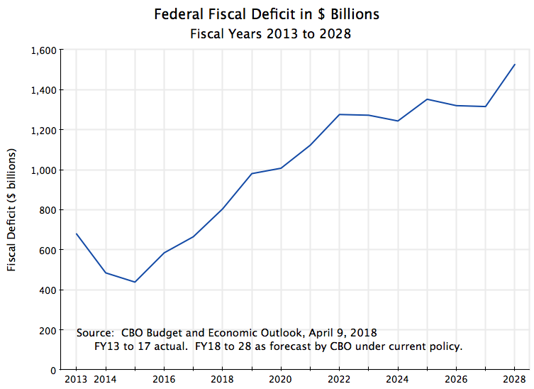
The total effect of all this will thus be to increase the fiscal deficit by $1.6 trillion over the ten years, over what it would otherwise have been.  The resulting annual fiscal deficits, in billions of dollars, would be as shown in the chart at top of this post.  Under the assumed scenario that the economy will remain at full employment over the entire period, the fiscal deficit will still rise to reach almost $1 trillion in FY19, and then to over $1.5 trillion in FY28.  Such deficits are unprecedented for when the economy is at full employment.

The deficits forecast would then translate into these shares of GDP, given the GDP forecasts:

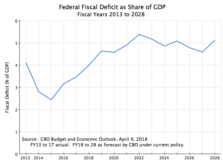
The CBO is forecasting that fiscal deficits will rise to a range of 4 1/2 to 5 1/2% of GDP from FY2019 onwards.  Again, this is unprecedented for the US economy in times of full employment.

C.  Fiscal Policy Over the Course of the Business Cycle

As noted above, fiscal policy has an important role to play during economic downturns to stabilize conditions and to launch a recovery.  When something causes an economic downturn (such as the decision during the Bush II administration not to regulate banks properly in the lead up to the 2008 collapse, believing “the markets” would do this best), both households and corporations will reduce their spending.  With unemployment increasing and wages often falling even for those fortunate enough to remain employed, as well as with the heightened general concerns on the economy, households will cut back on their spending.  Similarly, corporations will seek to conserve cash in the downturns, and will cut back on their spending both for the inputs they would use for current production (they cannot sell all of their product anyway) and for capital investments (their production facilities are not being fully used, so why add to capacity).

Only government can sustain the economy in such times, stopping the downward spiral through its spending.  Fiscal stimulus is needed, and the Obama stimulus program passed early in his first year succeeded in pulling the economy out of the freefall it was in at the time of his inauguration.  GDP fell at an astounding 8.2% annual rate in the fourth quarter of 2008 and was still crashing in early 2009 as Obama was being sworn in.  It then stabilized in the second quarter of 2009 and started to rise in the third quarter.  The stimulus program, as well as aggressive action by the Federal Reserve, accounts for this turnaround.

But fiscal deficits will be high during such economic downturns.  While any stimulus programs will add to this, most of the increase in the deficits in such periods occur automatically, primarily due to lower tax revenues in the downturn.  Incomes and employment are lower, so taxes due will be lower.  There is also, but to a much smaller extent, some automatic increase in government spending during the downturns, as funds are paid out in unemployment insurance or for food stamps for the increased number of the poor.  The deficits will then add to the public debt, and the public debt to GDP ratio will rise sharply (exacerbated in the short run by the lower GDP as well).

One confusion, sometimes seen in news reports, should be clarified.  While fiscal deficits will be high in a downturn, for the reasons noted above, and any stimulus program will add further to those deficits, one should not equate the size of the fiscal deficit with the size of the stimulus.  They are two different things.  For example, normally the greatest stimulus, for any dollar of expenditures, will come from employing directly blue-collar workers in some government funded program (such as to build or maintain roads and other such infrastructure).  A tax cut focused on the poor and middle classes, who will spend any extra dollar they receive, will also normally lead to significant stimulus (although probably less than via directly employing a worker).  But a tax cut focused on the rich will provide only limited stimulus as any extra dollar they receive will mostly simply be saved (or used to pay down debt, which is economically the same thing).  The rich are not constrained in how much they can spend on consumption by their income, as their income is high enough to allow them to consume as much as they wish.

Each of these three examples will add equally to the fiscal deficit, whether the dollar is used to employ workers directly, to provide a tax cut to the poor and middle classes, or to provide a tax cut to the rich.  But the degree of stimulus per dollar added to the deficit can be dramatically different.  One cannot equate the size of the deficit to the amount of stimulus.

Deficits are thus to be expected, and indeed warranted, in a downturn.  But while the resulting increase in public debt is to be expected in such conditions, there must also come a time for the fiscal deficits to be reduced to a level where at least the debt to GDP ratio, if not the absolute level of the debt itself, will be reduced.  Debt cannot be allowed to grow without limit.  And the time to do this is when the economy is at full employment.  It was thus the height of fiscal malpractice for the tax bills and budget passed by Congress and signed into law by Trump not to provide for this, but rather for the precise opposite.  The CBO estimates show that deficits will rise rather than fall, even under a scenario where the economy is assumed to remain at full employment.

It should also be noted that the deficit need not be reduced all the way to zero for the debt to GDP ratio to fall.  With a growing GDP and other factors (interest rates, the rate of inflation, and the debt to GDP ratio) similar to what they are now, a good rule of thumb is that the public debt to GDP ratio will fall as long as the fiscal deficit is around 3% of GDP or less.  But the budget and tax bills of Trump and the Congress will instead lead to deficits of around 5% of GDP.  Hence the debt to GDP ratio will rise.

[Technical note for those interested:  The arithmetic of the relationship between the fiscal deficit and the debt to GDP ratio is simple.  A reasonable forecast, given stated Fed targets, is for an interest rate on long-term public debt of 4% and an inflation rate of 2%.  This implies a real interest rate of 2%.  With real GDP also assumed to grow in the CBO forecast at 2% a year (from 2017 to 2028), the public debt to GDP ratio will be constant if what is called the “primary balance” is zero (as the numerator, public debt, will then grow at the same rate as the denominator, GDP, each at either 2% a year in real terms or 4% a year in nominal terms) .  The primary balance is the fiscal deficit excluding what is paid in interest on the debt.  The public debt to GDP ratio, as of the end of FY17, was 76.5%.  With a nominal interest rate of 4%, this would lead to interest payments on the debt of 3% of GDP.  A primary balance of zero would then imply an overall fiscal deficit of 3% of GDP.  Hence a fiscal deficit of 3% or less, with the public debt to GDP ratio roughly where it is now, will lead to a steady debt to GDP ratio.

More generally, the debt to GDP ratio will be constant whenever the rate of growth of real GDP matches the real interest rate, and the primary balance is zero.  In the case here, the growth in the numerator of debt (4% in nominal terms, or 2% in real terms when inflation is 2%) matches the growth in the denominator of GDP (2% in real terms, or 4% in nominal terms), and the ratio will thus be constant.]

Putting this in a longer-term context:

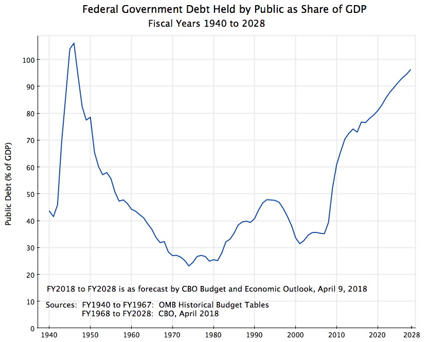
Federal government debt rose to over 100% of GDP during World War II.  The war spending was necessary.  But it did not then doom the US to perpetual economic stagnation or worse.  Rather, fiscal deficits were kept modest, the economy grew well, and over the next several decades the debt to GDP ratio fell.

For the fiscal balances over this period (with fiscal deficits as negative and fiscal surpluses as positive):

Fiscal balances were mostly but modestly in deficit (and occasionally in surplus) through the 1950s, 60s, and 70s.  The 3% fiscal deficit rule of thumb worked well, and one can see that as long as the fiscal deficit remained below 3% of GDP, the public debt to GDP ratio fell, to a low of 23% of GDP in FY1974.  It then stabilized at around this level for a few years, but reversed and started heading in FY1982 after Reagan took office.  And it kept going up even after the economy had recovered from the 1982 recession and the country was back to full employment, as deficits remained high following the Reagan tax cuts.

The new Clinton budgets, along with the tax increase passed in 1993, then stabilized the accounts, and the economy grew strongly.  The public debt to GDP ratio, which had close to doubled under Reagan and Bush I (from 25% of GDP to 48%), was reduced to 31% of GDP by the year Clinton left office.   But it then started to rise again following the tax cuts of Bush II (plus with the first of the two recessions under Bush II).  And it exploded in 2008/2009, at the end of Bush II and the start of Obama, as the economy plunged into the worst economic downturn since the Great Depression.

The debt to GDP ratio did stabilize, however, in the second Obama term, and actually fell slightly in FY2015 (when the deficit was 2.4% of GDP).  But with the deficits now forecast to rise to the vicinity of 5% of GDP (and to this level even with the assumption that there will not be an economic downturn at some point), the public debt to GDP ratio will soon be approaching 100% of GDP.

This does not have to happen.  As noted above, one need not bring the fiscal deficits all the way down to zero.  A fiscal deficit kept at around 3% of GDP would suffice to stabilize the public debt to GDP ratio, while something less than 3% would bring it down.

D.  Historical Norms

What stands out in these forecasts is how much the deficits anticipated now differ from the historical norms.  The CBO report has data on the deficits going back to FY1968 (fifty years), and these can be used to examine the relationship with unemployment.  As discussed above, one should expect higher deficits during an economic downturn when unemployment is high.  But these deficits then need to be balanced with lower deficits when unemployment is lower (and sufficiently low when the economy is at or near full employment that the public debt to GDP ratio will fall).

A simple scatter-plot of the fiscal balance (where fiscal deficits are a negative balance) versus the unemployment rate, for the period from FY1968 to now and then the CBO forecasts to FY2028, shows:

While there is much going on in the economy that affects the fiscal balance, this scatter plot shows a surprisingly consistent relationship between the fiscal balance and the rate of unemployment.  The red line shows what the simple regression line would be for the historical years of FY1968 to FY2016.  The scatter around it is surprisingly tight.  [Technical Note:  The t-statistic is 10.0, where anything greater than 2.0 is traditionally considered significant, and the R-squared is 0.68, which is high for such a scatter plot.]

An interesting finding is that the high deficits in the early Obama years are actually very close to what one would expect given the historical norm, given the unemployment rates Obama faced on taking office and in his first few years in office.  That is, the Obama stimulus programs did not cause the fiscal deficits to grow beyond what would have been expected given what the US has had in the past.  The deficits were high because unemployment was high following the 2008 collapse.

At the other end of the line, one has the fiscal surpluses in the years FY1998 to 2000 at the end of the Clinton presidency.  As noted above, the public debt to GDP ratio stabilized soon after Clinton took office (in part due to the tax increases passed in 1993), with the fiscal deficits reduced to less than 3% of GDP.  Unemployment fell to below 5% by mid-1997 and to a low of 3.8% in mid-2000, as the economy grew well.  By FY1998 the fiscal accounts were in surplus.  And as seen in the scatter plot above, the relationship between unemployment and the fiscal balance was close in those years (FY1998 to 2000) to what one would expect given the historical norms for the US.

But the tax cuts and budget passed by Congress and signed by Trump will now lead the fiscal accounts to a path far from the historical norms.  Instead of a budget surplus (as in the later Clinton years, when the unemployment rate was similar to what the CBO assumes will hold for its scenario), or even a deficit kept to 3% of GDP or less (which would suffice to stabilize the debt to GDP ratio), deficits of 4 1/2 to 5 1/2 % of GDP are foreseen.  The scatter of points for the fiscal deficit vs. unemployment relationship for 2018 to 2028 is in a bunch by itself, down and well to the left of the regression line.  One has not had such deficits in times of full employment since World War II.

E.  Conclusion

Fiscal policy is being mismanaged.  The economy reached full employment by the end of the Obama administration, fiscal deficits had come down, and the public debt to GDP ratio had stabilized.  There was certainly more to be done to bring down the deficit further, and with the aging of the population (retiring baby boomers), government expenditures (for Social Security and especially for Medicare and other health programs) will need to increase in the coming years.  Tax revenues to meet such needs will need to rise.

But the Republican-controlled Congress and Trump pushed through measures that will do the opposite.  Taxes have been cut dramatically (especially for corporations and rich households), while the budget passed in March will raise government spending (especially for the military).  Even assuming the economy will remain at full employment with no downturn over the next decade (which would be unprecedented), fiscal deficits will rise to around 5% of GDP.  As a consequence, the public debt to GDP ratio will rise steadily.

This is unprecedented.  With the economy at full employment, deficits should be reduced, not increased.  They need not go all the way to zero, even though Clinton was able to achieve that.  A fiscal deficit of 3% of GDP (where it was in the latter years of the Obama administration) would stabilize the debt to GDP ratio.  But Congress and Trump pushed through measures to raise the deficit rather than reduce it.

This leaves the economy vulnerable.  There will eventually be another economic downturn.  There always is one, eventually.  The deficit will then soar, as it did in 2008/2009, and remain high until the economy fully recovers.  But there will then be pressure not to allow the debt to rise even further.  This is what happened following the 2010 elections, when the Republicans gained control of the House.  With control over the budget, they were able to cut government spending even though unemployment was still high.  Because of this, the pace of the recovery was slower than it need have been.  While the economy did eventually return to full employment by the end of Obama’s second term, unemployment remained higher than should have been the case for several years as a consequence of the cuts.

At the next downturn, the fiscal accounts will be in a poor position to respond as they need to in a crisis.  Public debt, already high, will soar to unprecedented levels, and there will be arguments from conservatives not to allow the debt to rise even further.  Recovery will then be even more difficult, and many will suffer as a result.

Taxes to Pay for Highways: A Switch from the Tax on Gallons of Fuel Burned to a Tax on Miles Driven Would Be Stupid

Impact of Switching from Fuel Tax on Gallons Burned to Tax on Miles Driven

A.  Introduction

According to a recent report in the Washington Post, a significant and increasing number of state public officials and politicians are advocating for a change in the tax system the US uses to support highway building and maintenance.  The current system is based on a tax on gallons of fuel burned, and the proposed new system would be based on the number of miles a car is driven.  At least four East Coast states are proposing pilots on how this might be done, some West Coast states have already launched pilots, and states are applying for federal grants to consider the change.  There is indeed even a lobbying group based in Washington now advocating it:  The Mileage-Based User Fee Alliance.

There is no question that the current federal gas tax of 18.4 cents per gallon of gasoline is woefully inadequate.  It was last changed in 1993, 23 years ago, and has been kept constant in nominal terms ever since.  With general prices (based on the CPI) now 65% higher, 18.4 cents now will only buy 11.2 cents at the prices of 1993, a decline of close to 40%.  As a result, the Highway Trust Fund is terribly underfunded, and with all the politics involved in trying to find other sources of funding, our highways are in terrible shape. Basic maintenance is simply not being done.

An obvious solution would be simply to raise the gas tax back at least to where it was before in real terms.  Based on where the tax was when last set in 1993 and on the CPI for inflation since then, this would be 30.3 cents per gallon now, an increase of 11.9 cents from the current 18.4 cents per gallon.  Going back even further, the gasoline tax was set at 4 cents per gallon in 1959, to fund the construction of the then new Interstate Highway system (as well as for general highway maintenance).  Adjusting for inflation, that tax would be 32.7 cents per gallon now.  Also, looking at what the tax would need to be to fund adequately the Highway Trust Fund, a Congressional Budget Office report issued in 2014 estimated that a 10 to 15 cent increase (hence 28.4 cents to 33.4 cents per gallon) would be needed (based on projections through 2024).

These fuel tax figures are all similar.  Note also that while some are arguing that the Highway Trust Fund is underfunded because cars are now more fuel efficient than before, this is not the case.  Simply bringing the tax rate back in real terms to where it was before (30.3 cents based on the 1993 level or 32.7 cents based on the 1959 level) would bring the rate to within the 28.4 to 33.4 cents range that the CBO estimates is needed to fully fund the Highway Trust Fund.  The problem is not fuel efficiency, but rather the refusal to adjust the per gallon tax rate for inflation.

But Congress has refused to approve any such increase.  Anti-tax hardliners simply refuse to consider what they view as an increase in taxes, even though the measure would simply bring them back in real terms to where they were before.  And it is not even true that the general population is against an increase in the gas tax.  According to a poll sponsored by the Mineta Transportation Institute (a transportation think tank based at San Jose State University in California), 75% of those polled would support an immediate increase in the gas tax of 10 cents a gallon if the funds are dedicated to maintenance of our streets, roads, and highways (see the video clip embedded in the Washington Post article, starting at minute 3:00).

In the face of this refusal by Congress, some officials are advocating for a change in the tax, from a tax per gallon of fuel burned to a new tax per mile each car is driven.  While I do not see how this would address the opposition of the anti-tax politicians (this would indeed be a totally new tax, not an adjustment in the old tax to keep it from falling in real terms), there appears to be a belief among some that this would be accepted.

But even if such a new tax were viewed as politically possible, it would be an incredibly bad public policy move to replace the current tax on fuel burned with such a tax on miles driven.  It would in essence be a tax on fuel efficiency, with major distributional (as well as other) consequences, favoring those who buy gas guzzlers.  And as it would encourage the purchase of heavy gas guzzlers (relative to the policy now in place), it would also lead to more than proportional damage to our roads, meaning that road conditions would deteriorate further rather than improve.

This blog post will discuss why such consequences would follow.  To keep things simple, it will focus on the tax on gasoline (which I will sometimes simply referred to as gas, or as fuel).  There are similar, but separate taxes, on diesel and other fuels, and their levels should be adjusted proportionally with any adjustment for gasoline.  There is also the issue of the appropriate taxes to be paid by trucks and other heavy commercial vehicles.  That is an important, but separate, issue, and is not addressed here.

B.  The Proposed Switch Would Penalize Fuel Efficient Vehicles

The reports indicate that the policy being considered would impose a tax of perhaps 1.5 cents per mile driven in substitution for the current federal tax of 18.4 cents per gallon of gas burned (states have their own fuel taxes in addition, with these varying across states). For the calculations here I will take the 1.5 cent figure as the basis for the comparisons, even though no specific figure is as yet set.

First of all, it should be noted that at the current miles driven in the country and the average fuel economy of the stock of cars being driven, a tax of 1.5 cents per mile would raise substantially more in taxes than the current 18.4 cents per gallon of gas.  That is, at these rates, there would be a substantial tax increase.

Using figures for 2014, the average fuel efficiency (in miles per gallon) of the light duty fleet of motor vehicles in the US was 21.4 miles per gallon, and the average miles driven per driver was 13,476 miles.  At a tax of 1.5 cents per mile driven, the average driver would pay $202.14 (= $.015 x 13,476) in such taxes per year.  With an average fuel economy of 21.4 mpg, such a driver would burn 629.7 gallons per year, and at the current fuel tax of 18.4 cents per gallon, is now paying $115.87 (= $.184 x 629.7) in gas taxes per year. Hence the tax would rise by almost 75% ($202.14 / $115.87).  A 75% increase would be equivalent to raising the fuel tax from the current 18.4 cents to a rate of 32.1 cents per gallon.  While higher tax revenues are indeed needed, why a tax on miles driven would be acceptable to tax opponents while an increase in the tax per gallon of fuel burned is not, is not clear.

But the real reason to be opposed to a switch in the tax to miles driven is the impact it would have on incentives.  Taxes matter, and affect how people behave.  And a tax on miles driven would act, in comparison to the current tax on gallons of fuel burned, as a tax on fuel efficiency.

The chart at the top of this post shows how the tax paid would vary across cars of different fuel efficiencies.  It would be a simple linear relationship.  Assuming a switch from the current 18.4 cents per gallon of fuel burned to a new tax of 1.5 cents per mile driven, a driver of a highly fuel efficient car that gets 50 miles per gallon would see their tax increase by over 300%!  A driver of a car getting the average nation-wide fuel efficiency of 21.4 miles per gallon would see their tax increase by 75%, as noted above (and as reflected in the chart).  In contrast, someone driving a gas guzzler getting only 12 miles per gallon or less, would see their taxes in fact fall!  They would end up paying less under such a new system based on miles driven than they do now based on gallons of fuel burned.  Drivers of luxury sports cars or giant SUVs could well end up paying less than before, even with rates set such that taxes on average would rise by 75%.

Changing the tax structure in this way would, with all else equal, encourage drivers to switch from buying fuel efficient cars to cars that burn more gas.  There are, of course, many reasons why someone buys the car that they do, and fuel efficiency is only one.  But at the margin, changing the basis for the tax to support highway building and maintenance from a tax per gallon to a tax on miles driven would be an incentive to buy less fuel efficient cars.

C.  Other Problems

The change to a tax on miles driven from the tax on gallons of fuel burned would have a number of adverse effects:

a)  A Tax on Fuel Efficiency:  As noted above, this would become basically a tax on fuel efficiency.  More fuel efficient cars would pay higher taxes relative to what they do now, and there will be less of an incentive to buy more fuel efficient cars.  There would then be less of an incentive for car manufacturers to develop the technology to improve fuel efficiency.  This is what economists call a technological externality, and we all would suffer.

b)  Heavier Vehicles Cause Far More Damage to the Roads:  Heavier cars not only get poorer gas mileage, but also tear up the roads much more, leading to greater maintenance needs and expense.  Heavier vehicles also burn more fuel, but there is a critical difference.  As a general rule, vehicles burn fuel in proportion with their weight: A vehicle that weighs twice as much will burn approximately twice as much fuel.  Hence such a vehicle will pay twice as much in fuel taxes (when such taxes are in cents per gallon) per mile driven.

However, the heavier vehicle also cause more damage to the road over time, leading to greater maintenance needs.  And it will not simply be twice as much damage.  A careful early study found that the amount of damage from a heavier vehicle increases not in direct proportion to its weight, but rather approximately according to the fourth power of the ratio of the weights.  That is, a vehicle that weighs twice as much (for the same number of axles distributing the weight) will cause damage equal to 2 to the fourth power (=16) times as much as the lighter vehicle.  Hence if they were to pay taxes proportionate to the damage they do, a vehicle that is twice as heavy should pay 16 times more in taxes, not simply twice as much.

(Note that some now argue that the 2 to the fourth power figure found before might be an over-estimate, and that the relationship might be more like 2 to the third power.  But this would still imply that a vehicle that weighs twice as much does 8 times the damage (2 to the third power = 8).  The heavier vehicle still accounts for a grossly disproportionate share of damage to the roads.)

A tax that is set based on miles driven would tax heavy and light vehicles the same.  This is the opposite of what should be done:  Heavy vehicles cause far more damage to the roads than light vehicles do.  Encouraging heavy, fuel-thirsty, vehicles by switching from a tax per gallon of fuel burned to a tax per mile driven will lead to more road damage, and proportionately far more cost than what would be collected in highway taxes to pay for repair of that damage.

c)  Impact on Greenhouse Gases:  One also wants to promote fuel efficiency because of the impact on greenhouse gases, and hence global warming, from the burning of fuels. By basic chemistry, carbon dioxide (CO2) is a direct product of fuel that is burned.  The more fuel that is burned, the more CO2 will go up into the air and then trap heat. Economists have long argued that the most efficient way to address the issue of greenhouse gases being emitted would be to tax them in proportion to the damage they do.  A tax on gallons of fuel that are burned will do this, while a tax on miles driven (and hence independent of the fuel efficiency of the vehicle) will not.

An interesting question is what level of gasoline tax would do this.  That is, what would the level of fuel tax need to be, for that tax to match the damage being done through the associated emission of CO2.  The EPA has come up with estimates of what the social cost of such carbon emissions are (and see here for a somewhat more technical discussion of its estimates).  Unfortunately, given the uncertainties in any such calculations, as well as uncertainty on what the social discount rate should be (needed to discount costs arising in the future that follow from emitting greenhouse gases today), the cost range is quite broad. Hence the EPA presents figures for the social cost of emitting CO2 using expected values at alternative social discount rates of 2.5%, 3%, and 5%, as well as from a measure of the statistical distribution of one of them (the 95th percentile for the 3% discount rate, meaning there is only an estimated 5% chance that the cost will be higher than this).  The resulting costs per metric ton of CO2 emitted then range from a low of $11 for the expected value (the 50th percentile) at the 5% discount rate, $36 at the expected value for the 3% discount rate, and $56 for the expected value for the 2.5% discount rate, to $105 for the 95th percentile at a 3% discount rate (all for 2015).

With such range in social costs, one should be cautious in the interpretation of any one. But it may still be of interest to calculate how this would translate into a tax on gasoline burned by automobiles, to see if the resulting tax is “in the ballpark” of what our fuel taxes are or should be.  Every gallon of gasoline burned emits 19.64 pounds of CO2.  There are 2,204.62 pounds in a metric ton, so one gallon of gas burned emits 0.00891 metric tons of CO2.  At the middle social cost of $36 per metric ton of CO2 emitted (the expected value for the 3% social discount rate scenario), this implies that a fuel tax of 32.1 cents per gallon should be imposed.  This is surprisingly almost precisely the fuel tax figure that all the other calculations suggest is warranted.

d)  One Could Impose a Similar Tax on Electric Cars:  One of the arguments of the advocates of a switch from taxes on fuel burned to miles driven is that as cars have become more fuel efficient, they pay less (per mile driven) in fuel taxes.  This is true.  But as generally lighter vehicles (one of the main ways to improve fuel economy) they also cause proportionately far less road damage, as discussed above.

There is also an increasing share of electric, battery-powered, cars, which burn no fossil fuel at all.  At least they do not burn fossil fuels directly, as the electricity they need to recharge their batteries come from the power grid, where fossil fuels dominate.  But this is still close to a non-issue, as the share of electric cars among the vehicles on US roads is still tiny.  However, the share will grow over time (at least one hopes).  If the share does become significant, how will the cost of building and maintaining roads be covered and fairly shared?

The issue could then be addressed quite simply.  And one would want to do this in a way that rewards efficiency (as different electric cars have different efficiencies in the mileage they get for a given charge of electricity) rather than penalize it.  One could do this by installing on all electric cars a simple meter that keeps track of how much it receives in power charges (in kilowatt-hours) over say a year.  At an annual safety inspection or license renewal, one would then pay a tax based on that measure of power used over the year.  Such a meter would likely have a trivial cost, of perhaps a few dollars.

Note that the amounts involved to be collected would not be large.  According to the 2016 EPA Automobile Fuel Economy Guide (see page 5), all-electric cars being sold in the US have fuel efficiencies (in miles per gallon equivalent) of over 100 mpg, and as high as 124 mpg.  These are on the order of five times the 21.4 average mpg of the US auto stock, for which we calculated that the average tax to be paid would be $202.  Even ignoring that the electric cars will likely be driven for fewer miles per year than the average car (due to their shorter range), the tax per year commensurate with their fuel economy would be roughly $40.  This is not much.  It is also not unreasonable as electric cars are kept quite light (given the limits of battery technology) and hence do little road damage.

e)  There Are Even Worse Policies That Have Been Proposed:  As discussed above, there are many reasons why a switch from a tax on fuel burned to miles driven would be a bad policy change.  But it should be acknowledged that some have proposed even worse. One example is the idea that there should be a fixed annual tax per registered car that would fund what is needed for highway building and maintenance.  Some states in fact do this now.

The amounts involved are not huge.  As was calculated above, at the current federal gasoline tax of 18.4 cents per gallon, the driver of a car that gets the average mileage (of 21.4 mpg) for the average distance a year (of 13,476 miles) will pay $115.87 a year.  If the fuel tax were raised to 32.1 cents per gallon (or equivalently, if there were a tax of 1.5 cents per mile driven), the average tax paid would be still just $202.14 per year.  These are not huge amounts.  One could pay them as part of an annual license renewal.

But the tax structured in this way would then be the same for a driver who drives a fuel efficient car or a gas guzzler.  And it would be the same for a driver who drives only a few miles each year, or who drives far more than the average each year.  The driver of a heavy gas guzzler, or one who drives more miles each year than others, does more damage to the roads and should pay more to the fund that repairs such damage and develops new road capacity.  The tax should reflect the costs they are imposing on society, and a fixed annual fee does not.

f)  The Cost of Tax Collection Needs to be Recognized:  Finally, one needs to recognize that it will cost something to collect the taxes.  This cost will be especially high for a tax on miles driven.

The current system, of a tax on fuel burned, is efficient and costs next to nothing to collect.  It can be charged at the point where the gasoline and other fuels leaves in bulk from the refinery, as all of it will eventually be burned.  While the consumer ultimately pays for the tax when they pump their gas, the price being charged at the pump simply reflects the tax that had been charged at an earlier stage.

In contrast, a tax on miles driven would need to be worked out at the level of each individual car.  And if the tax is to include shares that are allocating to different states, the equipment will need to keep track of which states the car is being driven in.  As the Washington Post article on a possible tax on miles driven describes, experiments are underway on different ways this might be done.  All would require special equipment to be installed, with a GPS-based system commonly considered.

Such special equipment would have a cost, both up-front for the initial equipment and then recurrent if there is some regular reporting to the center (perhaps monthly) of miles driven.  No one knows right now what such a system might cost if it were in mass use, but one could easily imagine that a GPS tracking and reporting system might cost on the order of $100 up front, and then several dollars a month for reporting.  This would be a significant share of a tax collection that would generate an average of just $202 per driver each year.

There is also the concern that any type of GPS system would allow the overseers to spy on where the car was driven.  While this might well be too alarmist, and there would certainly be promises that this would not be done, some might not be comforted by such promises.

D.  Conclusion

While one should always consider whether given policies can be changed for the better, one needs also to recognize that often the changes proposed would make things worse rather than better.  Switching the primary source of funding for highway building and maintenance from a tax on fuel burned to a tax on miles driven is one example.  It would be a stupid move.

There is no doubt that the current federal tax on gasoline of 18.4 cents per gallon is too low.  The result is insufficient revenues for the Highway Trust Fund, and we end up with insufficient road capacity and roads that are terribly maintained.

What I was surprised by in the research for this blog post was finding that a wide range of signals all pointed to a similar figure for what the gasoline tax should be. Specifically:

  1. The 1959 gas tax of 4 cents per gallon in terms of current prices would be 32.7 cents per gallon;
  2. The 1993 gas tax of 18.4 cents per gallon in terms of current prices would be 30.3 cents per gallon;
  3. The proposal of a 1.5 cent tax per mile driven would be equivalent (given current average car mileage and the average miles driven per year) to 32.1 cents per gallon;
  4. The tax to offset the social cost of greenhouse gas emissions from burning fuel would be (at a 3% social discount rate) 32.1 cents per gallon.
  5. The Congressional Budget Office projected that the gasoline tax needed to fully fund the Highway Trust Fund would be in the range of 28.4 to 33.4 cents per gallon.

All these point in the same direction.  The tax on gasoline should be adjusted to between 30 and 33 cents per gallon, and then indexed for inflation.

The Tax Plans of the Republican Presidential Candidates Are Not Even Close to Serious

TPC Evaluations of Tax Losses in the Republican Tax Plans, 2016

A.  Introduction

There is a good deal in the current campaign of candidates seeking the Republican presidential campaign that is worrying.  When one of the main remaining candidates (Marco Rubio) tries to belittle one of the other candidates (Donald Trump) on national television by alluding to the size of his penis, one has to wonder.  This would be considered juvenile even in a campaign for a high school class president.  Yet one of these candidates will almost certainly receive the nomination of the Republican Party to be the President of the United States.

This blog seeks, however, to focus on economic issues.  And a key economic issue in modern day political campaigns is what the candidate would seek to do, if elected to office, about tax policy.  Major candidates have therefore set out detailed proposals while campaigning, with these proposals developed by teams of trusted advisors who are specialists in the area, and then put out by the candidate as what he (or she) would try to enact if elected.

The major Republican candidates have done this, and four of these (the proposals of Donald Trump, Ted Cruz, Marco Rubio, and Jeb Bush) have been analyzed in depth by the non-partisan Tax Policy Center (a joint center sponsored by the Urban Institute and the Brookings Institution).  (The Tax Policy Center has also just recently issued similar analyses of the tax plans of Hillary Clinton and Bernie Sanders.)

Among the issues examined by the Tax Policy Center was what the impact would be on revenues collected of the Republican plans.  This blog post will look at those estimates, and calculate what they imply for government expenditure cuts if, as each of the candidates insist, they would not allow deficits to rise.  And what they imply is that these plans, like much else in this campaign, simply are not serious.

B.  The Revenue Losses from the Republican Plans

The chart at the top of this post shows what the Tax Policy Center calculates the government revenue losses would be if the tax plans of the major Republican candidates were implemented.  Ten year totals (for fiscal years 2017 to 2026) are shown rather than year by year numbers to keep things simple, even though the plans would still be ramping up in 2017 with the full impact not seen until 2018.  The total revenue losses would range from $6.8 trillion for Bush as well as Rubio, to $8.6 trillion for Cruz, to $9.5 trillion for Trump.

To put this in perspective, the chart includes (on the right) the projected total government discretionary budget expenditures for all purposes other than defense over this same ten year period.  The figures are from the most recent (January 2016) ten year budget forecasts of the Congressional Budget Office, and will exclude defense as well expenditures for mandatory programs (two-thirds of which are for Social Security and Medicare) and for interest on public debt.

Forecast non-defense discretionary expenditures total $6.5 trillion over this ten year period.  This is less than what the revenue losses would be under any of the Republican plans.  That is, even with the total elimination of government discretionary spending on everything other than defense, the deficit would increase.  Yet these Republicans insist that their plans would not increase the deficit.

Cutting non-defense discretionary expenditures to zero is of course absurd.  For those concerned with security, one should note there would be no more federal prisons, no more prosecutors, no FBI, no more border control.  There would be no more federal disease control, no more federally funded medical research, no more federal support for infrastructure building or maintenance, no more NASA or supported science research, and so on.  Everything would be eliminated, not just cut.

Taking this a step further, one can look at how much defense spending would need to be cut, on top of the elimination of all non-defense expenditure, to make up for the lost revenues:

Implied Defense Reductions, FY2017 to 2026, TPC

The necessary cuts in the defense budget would range from 5% of forecast ten-year defense expenditures for Bush and Rubio, to 32% for Cruz, to 47% (!) for Trump.  Yet Cruz, Rubio and Bush have all also called for sharp increases in defense spending.  Ted Cruz has laid out an ambitious plan for a bigger military that an analyst at the conservative Cato Institute would cost an extra $2.6 trillion over eight years, an increase in defense spending of over 50%.  Bush and Kasich have each proposed increases in defense spending of $1 trillion over ten years, an increase of over 15%.  Rubio is also arguing for big (but unspecified) increases in defense spending.  Things are perhaps less clear for Donald Trump, who has asserted he is “gonna build a military that’s gonna be much stronger than it is right now”, but “for a lot less”.  How he would do this he does not say, and it is doubtful he would get a “much stronger” military if its budget is to be cut by close to half.

C.  Conclusion

The Republican candidates assert their tax cut plans would not, however, lead to deficit increases, nor that they would cut defense spending (at least other than Trump).  Rather, they would cut non-defense spending.  However, as seen above, even if non-defense spending were cut to zero, budget deficits would increase unless there were also sharp cuts in mandatory programs (which are mostly Social Security and Medicare).

How do they believe they can do this?  Because they assert their tax plans would lead to big, indeed miraculous, leaps in growth.  Yet there is no evidence that such tax plans would do this.  Indeed, they are so large that the disruption in finances would almost certainly have large negative consequences for growth.

Economic theory does suggest that tax systems can affect growth.  The Tax Policy Center evaluations of the Republican tax plans, cited above, each have a balanced discussion of what they might be.  But as they point out, one would expect from economic theory that there would be both positive and negative effects, offsetting each other to at least some degree, and that in any case the overall impact in either direction is likely to be small. What the net impact will be, and in what direction, is then an empirical question, and careful studies of historical examples of tax reforms suggests that the overall impact on growth is, indeed, small.

One also does not find any evidence in the US historical data that tax cuts lead to more rapid growth.  As an earlier post on this blog found, federal taxes as a share of GDP were substantially lower in the decade following the Bush tax cuts of 2001 than for any decade in the previous half century, but this was not associated with higher GDP or jobs growth. Rather, it was associated with the lowest growth of GDP or jobs of any decade since at least the 1960s.  Furthermore, one cannot find any indication that a reduction of the highest marginal income tax rate (a focus of the Republican tax plans) led to higher growth.  The highest marginal federal income tax rate was 91 or 92% in the 1950s under Eisenhower, and always 70% or higher during the 1960s, but growth in GDP and in jobs during those periods were reasonably good, especially in comparison to what they have been since the Bush tax cuts of 2001.  High marginal income tax rates in the 1950s and 1960s did not kill growth.

One should not then expect miracles.  The Republican tax plans simply cannot be taken seriously.  But perhaps I am being silly to expect that in this campaign for the presidency.