The Sluggish Recovery: Fiscal Drag Continues to Hold Back the Economy

Recessions - GDP Around Peak, 12Q before to 22Q after

I.  Introduction

The recovery from the 2008 economic collapse remains sluggish, with GDP growing in the first half of 2013 at an annualized rate of only 1.4% (according to recently released BEA estimates).  And based on fourth quarter to fourth quarter figures, GDP grew by only 2.0% in 2011 followed by just 2.0% again in 2012.  As a result, the unemployment rate has come down only slowly, from a peak of 10.0% in 2009 to a still high 7.4% as of July.

Conservatives have asserted that the recovery has been slow due to huge and unprecedented increases in government spending during Obama’s term, and that the answer should therefore be to cut that spending.  But as has been noted in earlier posts on this blog, direct government spending during Obama’s term has instead been falling.  This reduction in demand for what the economy can produce has slowed the recovery from what it would have been.

This blog will update numbers first presented in a March 2012 post on this blog, which compared the paths of GDP, government spending, and other items in the periods before and after the start of each of the recessions the US has faced since the 1970s.  That earlier blog post looked at the paths of GDP and the other items from 12 quarters before the business cycle peak (as dated by the NBER, the entity that organizes a panel of experts to date economic downturns) to 16 quarters after those peaks (when the downturns by definition begin).  The figures were rebased to equal 100.0 at the business cycle peaks.  We now have an additional year and a half of GDP account data, so it is now possible to extend the paths to 22 quarters from the start of the recent downturn in December 2007.  This has therefore been done for all.

The conclusions from the earlier post unfortunately remain, but are even more clear with the additional year and a half of observations.  GDP growth remains sluggish, government spending has fallen by even more, and residential investment remains depressed (although it has finally begun to recover).

II.  The Path of Real GDP

The graph at the top of this post shows the path followed by real GDP in the periods from 12 quarters before to 22 quarters after the onset dates of each of the recessions the US has faced since the 1970s.  The sluggish recovery from the current downturn is clear.

The economy fell sharply in the final year of the Bush administration, and then stabilized quickly after Obama took office.  GDP then began to grow from the third quarter of 2009 and has continued to grow since.  But the pace of recovery has been slow.  By 22 quarters from the previous business cycle peak, real GDP in the current downturn is only 4% above where it had been at that peak.  At the same point in the other downturns since the 1970s, real GDP was between 15% and 20% above where it had been at the previous peak.  This has been a terrible recovery.

 III.  The Path of Government Spending

How has this recovery differed from the others?  To start to understand this, look at the path government spending has taken:

Recessions - Govt Cons + Inv Expenditures Around Peak, 12Q before to 22Q after

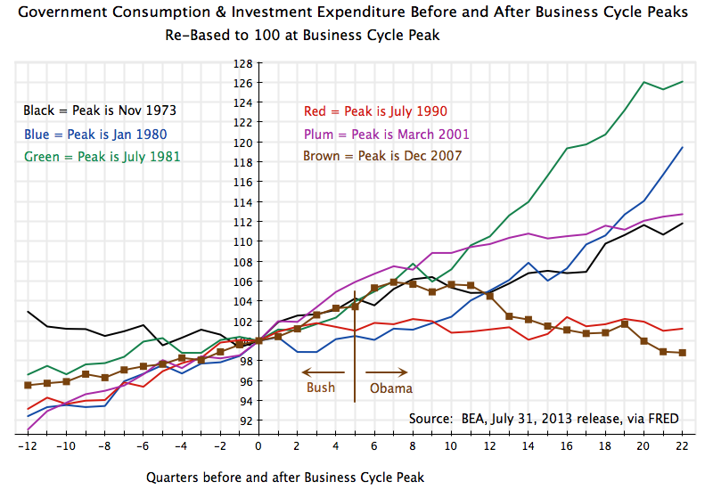
Direct government spending has fallen in this recovery, in sharp contrast to the increases seen in the other recoveries.  Real government spending was 26% higher by 22 quarters after the onset of the July 1981 recession (the green line) during the Reagan presidency, and 13% higher at the same point in the recovery from the March 2001 recession (the plum colored line) during the Bush II presidency.  While both Reagan and Bush claimed to represent small government conservatism, government spending instead rose sharply during their terms.

In contrast, in the current downturn direct government spending is now 1.2% below what it had been at the start of the recession in December 2007.  Furthermore, it is worth noting that while it rose in the final year of the Bush presidency and then in the first half year after Obama took office (a major reason why the recovery then began), it has since fallen sharply.  Government spending is now almost 7% below where it had been in mid-2009, a half year after Obama took office.  Such a decline (indeed no decline) has ever happened before, going back at least four decades, as the economy has struggled to recover from a recession.  The closest was during the Clinton years, when government spending was essentially flat (a 1% increase at the same point in the recovery).

Note that the measure of government spending shown here is that for total government spending on consumption and investment (i.e. all government spending on goods and services).  This is the direct component of GDP.  Government spending can also be measured by including transfer payments to households (such as for Social Security or unemployment insurance), but as was noted in the earlier blog post from March 2012, the results are similar.  Note also that the government spending figures include spending at the state and local levels, in addition to federal spending.  While we speak of government spending as taking place during some presidential term in office, the decisions are made not simply by the president but also by many others (including state and local officials, and the Congress) in the US system.  But the president at the time is typically assigned the blame (or the credit) for the outcome.

IV.  The Path of Residential Investment

The current downturn and recovery also differs from the others by the scale of the housing collapse, and consequent fall in residential investment:

Recessions - Residential Investment Around Peaks, 12Q before to 22Q after

The build up of the housing bubble from 2002 to 2006 was unprecedented in the US, and the collapse then more severe.  As the graph above shows, there has been a start in the recovery of residential investment from the lows it had reached in 2009 / 2010, but it is still far below the levels seen in previous downturns.

Housing had been overbuilt during the bubble in the Bush years, leaving an oversupply of housing once the bubble burst.  And while supply was in excess, demand for housing was reduced due to the severe recession.  As was discussed in an earlier blog post on the housing crisis, the result was a doubling up of households as well as delays in household formation as young adults continued to live with their parents.  Residential investment therefore collapsed, and has recovered only very slowly.

V.  The Path of Household Debt

The housing bubble also led to over-indebtedness of households.  Nothing of this sort at all close to this scale had ever happened before in the US.  With the lack of regulation and oversight of the financial sector during the Bush administration, banks and other financial entities launched and aggressively marketed and sold financial instruments that led to a bidding up of home prices.  But these new financial instruments were only viable if housing prices continued to rise forever.  When the housing bubble burst, widespread defaults followed.  And those households who did not default struggled to pay down the debts they had taken on, for assets now worth less than the size of the debts tied to them.

The result was a sustained fall in household debt (three-quarters of which is mortgage debt) in the period of the downturn:

Recessions - HH Debt Around Peak, 12Q before to 22Q after

This pay-down of debt had never happened before, and is in stark contrast to the rise in household debt seen in all the other downturns of the last four decades.

VI.  The Path of Personal Consumption Expenditure

Households struggling to pay down their debt have to cut back on their consumption expenditures.  This brings us to the last element of the current recovery I would like to highlight:  the especially slow recovery in household consumption.  That path of consumption during the current downturn stands out again in contrast to the paths followed in the other downturns and recoveries of the last four decades in the US:

Recessions - Personal Consumption Around Peaks, 12Q before to 22Q after

The difference is stark.  Households could spend more in the prior recoveries in part because they could continue to borrow (see the graph on household debt above).  In this recovery, households have instead had to pay down the debts they had accumulated in the housing bubble years, and could increase their household consumption only modestly.

VII.  Conclusion

The recovery in the current downturn has been disappointing.  GDP has grown since soon after Obama took office, but has grown only slowly, and has been on a path well below that seen in other recoveries.

There are a number of reasons for this.  Household consumption has kept to a low path as households have struggled to repay the over-indebtedness they had accumulated during the housing bubble years.  Residential investment collapsed as well following the bubble, is only now starting to recover, and remains far below the levels seen at similar points in other recoveries.
And government spending has been allowed to fall during Obama’s term.  This had never happened before in the previous downturns.  Indeed, while real government spending rose by 26% at the same point in the economic recovery during the Reagan presidency, it has been reduced by over 1% in this recovery (and reduced by 7% from what it had been a half year after Obama took office).
The reduction in government spending reduced the demand for what the economy could have produced.  In this it was similar to the reduced demand resulting from lower residential investment or lower household consumption expenditure.  All these reductions in demand reduced GDP, reduced the demand for workers, and hence increased unemployment.  But while residential investment and household consumption can only be influenced indirectly and highly imperfectly by government policy, government has direct control over how much it spends.  That is, government can decide whether to build a road or a school building, and doing so will employ workers and will lead to an increase in GDP.  Hence government spending is a direct instrument that can be used to raise growth and employment, should the government so choose.
Sadly, and in stark contrast to the sharp increase in government spending during the Reagan period that spurred the recovery to the 1981 downturn, US politics during the Obama presidency have instead led to a cut-back in government spending, with a resulting drag on growth.  The disappointing consequences are clear.

Obama and Prices: The Markets Expect Inflation to Remain Low

US Treasury Bond Yields, TIPS, and Expected Inflation, Jan 2, 2003, to Aug 8, 2013

Conservative critics of Obama argue his policies will inevitably lead to high inflation.  A previous blog post on this site showed that in fact inflation during the four years of Obama’s first term had been the lowest over any presidential four year term going back a half century.  Low inflation during Obama’s first term cannot be denied.

The conservative critics respond that while inflation may have been low so far, it is inevitable that inflation will soon rise.  The blog post cited above provides links to several examples of what they have been saying.  But this assertion can be examined as well.  In particular, the financial markets (which the conservative critics generally take as reflecting a sound view on such matters, as the investment returns of such investors will depend on getting this right) can be used to see what at least the markets believe inflation will be going forward.

Since 1997 the US Treasury has been issuing bonds of varying maturities whose principal is indexed to the US CPI price index.  These bonds, known as TIPS (for Treasury Inflation-Protected Securities), provide a return which will be the same in real terms regardless of what inflation turns out to be.  The yields on such bonds can be compared to the yields on regular US Treasury bonds of similar maturity.  Such regular US Treasury bonds will pay interest and at the end return the principal in certain dollar amounts, with a value in real terms which will vary depending on what inflation turned out to be.

Inflation is normally positive, so the regular bonds will pay rates which are higher than the rates on TIPS bonds.  But whether the higher rates are worthwhile will depend on how high inflation turns out to be.  To illustrate with some simple numbers, suppose the rate on a 10-year regular US Treasury bond is 3% while the rate on a 10-year TIPS is 1%.  If inflation turns out to be 2%, the bonds will be equally valuable.  But if inflation turns out to be 3%, it would have been better to have invested in the TIPS.  The TIPS will still pay out a 1% real return, while the regular US Treasury will yield a real return of only 0% (a 3% nominal return, but with 3% inflation the real yield will be zero).  Alternatively, suppose inflation turns out to be 1%.  The real return on the regular US Treasury will be 2% (equal to 3% minus 1%), while the TIPS will still yield the contracted 1% real return.  In one believes inflation will be just 1% over this period until maturity, it would have been better to have invested in the regular bonds.

The investors will therefore need to determine what they expect inflation to be.  They will bid up the price of one of the bonds (and bid down the price of the other) if they believe inflation over the time to maturity of the bond, will be higher or lower than the current gap in the yields between the two.  Where the prices of the two bonds settle, and therefore what the gap in yields is between the two, therefore reflects what the financial markets as a whole believe will be the rate of CPI inflation over the period until the bonds mature.  Since real money is riding on this, the investors will take it seriously.

The graph above shows the yields on regular 10-year US Treasury bonds (in blue) and on 10-year TIPS (in green), for the period from January 2, 2003, to August 8, 2013.  The data comes from the official US Treasury web site (where the data presented there goes back to January 2, 2003).  The implied 10-year expected rate of inflation (in red) is then calculated based on the difference between the two yields.

As can be seen in the graph, the yields on the regular 10-year US Treasury bond varied a fair amount over the period, from generally between 4 and 5% during the Bush presidency, falling over time to below 2% for much of 2012, and then rising to about 2 1/2% recently.  The 10-year TIPS yield similarly varied from around 2% during the Bush years, to negative levels for 2012 and the first half of 2013, and rising to a still low but positive 1/2% recently (and most recently just 1/3%).

Despite such fluctuations in the yields of the regular 10-year bond and the 10-year TIPS, the implied expected inflation rate (the difference between the two yields) has been relatively constant, at about 2 1/2% during the Bush years and a similar but slightly lower rate (on average) during the Obama presidency.  The one exceptional period, which should be excluded, would be during the period of economic and financial collapse in the final months of the Bush presidency, after Lehman Brothers went bankrupt and the financial markets were in chaos.  The TIPS yields went up while the regular US Treasury bond yields fell sharply, leading to an implied expectation of inflation of close to zero.  But the figures under such chaotic conditions should not be taken as meaningful.  The chaotic markets then stabilized within a short period of Obama taking office in January 2009, with the rates then returning to more normal levels.

The financial markets, which the conservative critics of Obama normally place a good deal of faith in, therefore do not show any indication that they expect inflation over the next decade to rise.  Rather, they expect inflation of around 2% a year to continue, which is consistent also with the rate of inflation the Fed targets.

Finally, the figures on the bond yields in the graph above also show that the US government has been able to borrow, and continues to be able to borrow, at incredibly low rates, whether in real or nominal terms.   The TIPS yield (the borrowing rate in real terms) was indeed negative in for most of 2012 and the first half of 2013, and is still only 1/2% or less.  Even were it not for the still high unemployment in the country, this is the period when the government should be undertaking investments in both new infrastructure and other assets, and in maintenance of existing assets.  Such investments are worthwhile even if they generate returns of only 1/2% in real terms.  Yet such investments, particularly in maintenance, will generate returns that are orders of magnitude greater than that.

It has been incredibly stupid that the Republican insistence on cutting government spending has blocked us from proceeding with such investments at a time when the borrowing costs to fund them have been so low.

Impact of the 1994 Assault Weapons Ban on Homicide Rates and Mass Shootings

US Murder Rates, 1980 to 2010Mme. Marie Curie (Nobel Laureate):  “Nothing in life is to be feared, it is only to be understood.  Now is the time to understand more, so that we may fear less.”

[Note:  An update to this post, with more recent data as well as a discussion of what should be done for a more effective ban, was posted on this blog on March 17, 2018.]

Introduction

The horrific shootings at Sandy Hook Elementary in Connecticut in December, in which 20 school children aged 6 and 7 died, led to an outcry for effective measures to stop this from happening again.  The gun control measure most commonly called for was reinstatement of the ban on assault weapons (the type of weapon used in the Sandy Hook shooting) that Congress had passed in September 1994.  The law had a 10 year sunset provision, and with the more conservative political climate in 2004 during the Bush Administration, efforts to renew the law were blocked.  Hence it expired in September 2004.  The mother of the Sandy Hook shooter was then legally eligible to purchase an assault weapon, and her son used the one she had at their home to kill the 20 school children, after he first shot his mother.

But did the 1994 Assault Weapons Ban law have an effect on homicides in the US, and separately on mass shootings?  This note will review what we might be able to say from simple trends over time.

US Homicide Rates Fell in the 1990s

The chart above shows US homicide rates between 1980 and 2010, with a breakdown (for 1980 to 2008) of the number of homicides as a result of the use of any gun, by handguns only, and by all other guns.  Other homicides could be through the use of knives or other objects.  The source is a report dated November 2011 on homicide trends in the US over 1980 to 2008, prepared in the Bureau of Justice Statistics of the US Department of Justice, and is the most recent such report available from this source.

The chart shows that homicides did indeed decline sharply over the 1994 to 2004 period that the law was in effect (more precisely, September 13, 1994, to September 12, 2004).  The overall homicide rate in the US was 9.5 deaths per 100,000 population in 1993, and this fell to a rate of 5.6 in 2005.  The homicide rate from use of guns fell from 6.6 in 1993 to 3.8 in 2005.

While these homicide rates are an improvement over what they had been, keep in mind that compared to other developed countries, the rates are still abysmal.  Based on UN assembled data for 2010 (or the most recent year available), the total homicide rates were just 1.2, 0.8, 1.1, and 0.4 for the UK, Germany, France, and Japan respectively, and the homicide rates by firearms were only 0.1, 0.2, 0.1, and 0.0 for the four countries (where the rate in Japan rounded to 0.0 per 100,000 population as there were only 11 homicides in Japan in 2008, the most recent year with data available in the UN report on this; in 2008, the US had 11,030 homicide deaths by firearms.  Japan has strict gun controls.).

But can one attribute this fall in the homicide rate to be a consequence of the Assault Gun Ban then in effect?  From just the relationship found in the chart, not really.  There was much else going on during this period which could and probably did also have an impact on homicide rates.  In addition, one can see in the chart that the decline in homicide rates began before the new law went into effect, and that the large fall then bottomed out around 2000, after which there was a small rise.  Furthermore, one does not see a jump back to previous rates once the ban was allowed to expire in September 2004.  Looking at this relationship over time, a stronger case could probably be made that the drop in the homicide rate was more due to the totality of measures implemented during the period of the Clinton presidency, from January 1993 to January 2001.  This fits well the observed period when the homicide rate dropped.  But here again, there was much else also going on which could affect the homicide rates, including at the level of state and local governments.

Mass Shootings, 1982 to 2012

It is also arguable that the metric used above (the overall homicide rate) is not the metric that should be used when assessing whether the Assault Gun Ban helped.  The Assault Gun Ban only affected one category of gun (semi-automatic weapons), and highly imperfectly at that (which will be discussed below).  Most murders are done with simple handguns.  Particularly with the Sandy Hook shooting of school children very much in mind, can one say whether the 1994 Assault Gun Ban may have reduced the number of, and severity of, mass shootings?

Following the Sandy Hook shooting, Mother Jones magazine recently updated a data set it had earlier prepared (after the Aurora theater shootings) on mass shootings in the US since 1982.  Using specific criteria to define what to include as a mass shooting (four or more people shot in a single incident; one shooter; the shootings occurred in a public place; and some other factors and with some specified exceptions), Mother Jones provides a well documented data set concluding that there were 62 mass shootings meeting its criteria over this period.  They provide brief descriptions of each event, what weapons were used, the number of fatalities and the number of those wounded, and other relevant data.

Based on this data set, the following graph shows the number of mass shooting incidents in each year from 1982 to 2012:

Mass Shootings, Number by Year, 1982-2012

The number of mass shootings meeting the specified definition averaged 1.5 each year between 1982 and 1994, and possibly might have been rising in the period leading up to 1994 (I say possibly as the number of events are small, and it is not clear this is statistically significant).  The annual average was about the same, at 1.6 per year, between 1995 and 2004, but with this average brought up by a high number in 1999 (the year of the Columbine High School shooting, but where there were five mass shootings in total), and to a lesser extent in 1998 (with three mass shootings).  The numbers were low in the other years.  After the Assault Gun Ban expired, the frequency went up, reaching 3.4 per year on average between 2005 and 2012, with an especially high number (seven) in 2012.

The data set also has the numbers over time on the number of fatalities and of all victims (including those wounded):

Mass Shootings, Fatalities and Total Victims, 1982-2012

Using the numbers underlying this figure, over 1982 to 1994 the number of fatalities in mass shootings averaged 8.5 per year and the number of total victims (including those injured) averaged 18.2.  Over the period 1995 to 2004, the number of fatalities fell somewhat to 6.4 per year while the total number of victims fell to 13.2.  The averages were higher than otherwise in this period due to the spikes in 1999 (the year of Columbine) and to a lesser extent 1998.  The numbers then went higher in the period 2005 to 2012, after the Assault Weapons Ban expired, to 9.2 fatalities per year and 16.7 total victims per year.  2012 was a particularly bad year.

But with the limited number of years and small number of incidents involved each year, it is difficult to say whether there were significant changes over time, and in particular whether the fatalities fell significantly during the period the Assault Weapons Ban was in effect.  Were it not for 1999, and to a lesser extent 1998, the number of annual fatalities and victims would have fallen sharply during the period of the Assault Weapons Ban, and then risen again after it was abandoned.  But 1999 and 1998 did occur, so it is hard to say whether the impact was significant.

The underlying numbers also indicate that over the period as a whole, 73% of the weapons used in the mass shootings (and there were typically multiple weapons used in each mass shooting) were either semi-automatic handguns or long-barreled assault weapons.  Both were in principle banned under the Assault Weapons Ban, but only the manufacture and sale of new such weapons were banned –  the existing stock remained.  Such weapons accounted for 67% of the weapons used in the mass shootings between 1982 and 1994, for 74% of the weapons during the period of Assault Weapons Ban was in effect, and for essentially the same share of 75% in the period 2005 to 2012 when the law had expired.  There was no significant change during the period of the Assault Weapons Ban.

Limitations of the Assault Weapons Ban Law

The evidence is therefore not clear whether the 1994 Assault Weapons Ban had a significant effect.  But part of this is certainly a consequence of the “ban” being extraordinarily weak.  While the law was controversial, and some attribute the loss of the Congress by the Democrats to a resurgent Republican Party that year (when Newt Gingrich became Speaker) to passage of the act, the act itself did little to “ban” assault weapons, despite the title.

First of all, the law only affected the manufacture and subsequent sale of newly produced assault weapons.  The existing stock of such weapons would remain, and could be sold or transferred between owners.  In anticipation of the law, manufacturers flooded the market with a huge supply of newly produced weapons.  Second, the law defined “assault weapons” in a highly specific way.  As an advocacy group later noted, gun manufacturers soon found they could circumvent the law with what were little more than cosmetic changes to the existing arms.  Finally, while the Assault Weapons Ban also limited the manufacture and sale of newly produced high capacity ammunition magazines (limited to ten rounds or less), the manufacturers also ramped up production of these clips and flooded the market in the period before the law went into effect.  The high capacity clips were still widely available in 2004.

With these limitations in the law, it is not surprising that it is difficult to determine with any confidence whether the law had an effect on homicides and mass shootings.  And it appears as I write this, that President Obama is likely to propose tomorrow, January 16, a new assault weapons ban as a center piece of his initiative to reduce gun violence.  I would certainly welcome this.  But for the law to be effective, it will be very important that it take into account and remedy the limitations that made the 1994 Assault Weapons Ban so weak.  And I do not expect that the current Congress will do this.

The Need for Serious Analysis and Research

It is also clear that the limitations that have been placed on serious research on the causes of gun violence has to end.  These were discussed in a previous posting on this blog.  As discussed there (and also see a recent summary here), the limitations on research have been imposed by a conservative Congress at the instigation of the NRA.

A good recent summary of the problem is provided in an open letter to Vice President Biden (as chair of the Commission on Gun Violence) signed by a senior group of 108 professors and analysts from prominent universities and institutions.  Despite the importance of gun violence to our health, the US Centers for Disease Control and Prevention (CDC) has been effectively blocked from sponsoring research on understanding the issue, and the CDC and the US Bureau of Alcohol, Tobacco, Firearms, and Explosives (ATF) have not been allowed even to assemble and disseminate relevant data.

As a consequence, high level review commissions have been forced to say, honestly, that we simply do not know what the impact of various possible gun measures might be.  Comprehensive reviews in 2003 by the CDC and in 2004 by the National Research Council of the National Academies of Sciences had to conclude that the research has not been done, nor even the data assembled to permit such research to be done, to determine what might be effective in curbing gun violence.  And as the CDC report notes in its up front summary:  “insufficient evidence to determine effectiveness should not be interpreted as evidence of ineffectiveness.”  They both called for further work, but I am not aware of a similar commission and review since 2003/2004, which itself is indicative.

It is extremely important to keep in mind that while we do not have adequate analysis which can allow us to say with any certainty what measures might be taken to reduce gun violence, that does not mean that measures to control the availability of firearms will not be effective.  We do, after all, see the lower homicide rates, and especially the far lower homicide rates by firearms, in countries that have controlled access to firearms, such as most of Europe and Japan.  Figures are cited above.  And it is not true that the overall level of crime is especially high in the US.  According to statistics issued by the OECD, the overall crime rate in the US, as well as the rate of criminal assaults and threats, are in the middle of the ranges for the 26 OECD members reviewed.  Where the US stands out is not in criminality, but in homicides resulting from criminality.

The easy availability of guns certainly has something to do with this.

Update:  An observant reader noted that in my original post I had mistakenly referred to Sandy Hook Elementary as Sandy Hill Elementary.  I have corrected that in the above.  My thanks to that reader.