How Fast is GDP Growing?: A Curiosum

A.  How Fast is GDP Growing?

The Bureau of Economic Analysis released today its first estimate (what it calls it’s Advance Estimate) for the growth of GDP and its components for the third quarter of 2019.  Most of it looked basically as one would expect, with an estimate of real GDP growth of 1.9% in the quarter, or about the same as the 2.0% growth rate of the second quarter.  There has been a continued slowdown in private investment (which I will discuss below), but this has been offset by an expansion in government spending under Trump, coupled with steady growth in personal consumption expenditures (as one would expect with an economy now at full employment).

But there was a surprise on the last page of the report, in Appendix Table A.  This table provides growth rates of some miscellaneous aggregates that contribute to GDP growth, as well as their contribution to overall GDP growth.  One line shown is for “motor vehicle output”.  What is surprising is that the growth rate shown, at an annualized rate, is an astounding 32.6%!  The table also indicates that real GDP excluding motor vehicle output would have grown at just 1.2% in the quarter.  (I get 1.14% using the underlying, non-rounded, numbers, but these are close.)  The difference is shown in the chart above.

Some points should be noted.  While all these figures provided by the BEA are shown at annualized growth rates, one needs to keep in mind that the underlying figures are for growth in just one quarter.  Hence the quarterly growth will be roughly one-quarter of the annual rate, plus the effects of compounding.  For the motor vehicle output numbers, the estimated growth in the quarter was 7.3%, which if compounded over four quarters would yield the 32.6% annualized rate.  One should also note that the quarterly output figures of this sector are quite volatile historically, and while there has not been a change as large as the 32.6% since 2009/10 (at the time of the economic downturn and recovery) there have been a few quarters when it was in the 20s.

But what appears especially odd, but also possibly interesting to those trying to understand how the GDP accounts are estimated, is why there should have been such a tremendously high growth in the sector, of 32.6%, when the workers at General Motors were on strike for half of September (starting on September 15).  GM is the largest car manufacturer in the US, its production plummeted during the strike, yet the GDP figures indicate that motor vehicle output not only soared in the quarter, but by itself raised overall GDP growth to 1.9% from a 1.2% rate had the sector been flat.

This is now speculation on my part, but I suspect the reason stems from the warning the BEA regularly provides that the initial GDP estimates that are issued just one month after the end of the quarter being covered, really are preliminary and partial.  The BEA receives data on the economy from numerous sources, and a substantial share of that data is incomplete just one month following the end of a quarter.  For motor vehicle production, I would not be surprised if the BEA might only be receiving data for two months (July and August in this case), in time for this initial estimate.  They would then estimate the third month based on past patterns and seasonality.

But because of the strike, past patterns will be misleading.  Production at GM may have been ramped up in July and August in anticipation of the strike, and a mechanical extrapolation of this into September, while normally fine, might have been especially misleading this time.

I stress that this is speculation on my part.  Revised estimates of GDP growth in the third quarter, based on more complete data, will be issued in late November and then again, with even more data, in late December.  We will see what these estimates say.  I would not be surprised if the growth figure for GDP is revised substantially downwards.

B.  Growth in Nonresidential Private Fixed Investment

The figures released by the BEA today also include its estimates for private fixed investment.  The nonresidential portion of this is basically business investment, and it is interesting to track what it has been doing over the last few years.  The argument made for the Trump/Republican tax cuts pushed through Congress in December 2017 were that they would spur business investment.  Corporate profit taxes were basically cut in half.

But the figures show no spur in business investment following their taxes being slashed.  Nonresidential private fixed investment was growing at a relatively high rate already in the fourth quarter of 2017 (similar to rates seen between mid-2013 and mid-2014, and there even was growth of 11.2% in the second quarter of 2014).  This continued through the first half of 2018.  But growth since has fallen steadily, and is now even negative, with a decline of 3.0% in the third quarter of 2019:

There is no indication here that slashing corporate profit taxes (and other business taxes) led to greater business investment.

The “Threat” of Job Losses is Nothing New and Not to be Feared: Issues Raised in the Democratic Debate

A.  Introduction

The televised debate held October 15 between twelve candidates for the Democratic presidential nomination covered a large number of issues.  Some were clear, but many were not.  The debate format does not allow for much explanation or nuance.  And while some of the positions taken refected sound economics, others did not.

In a series of upcoming blog posts, starting with this one, I will review several of the issues raised, focussing on the economics and sometimes the simple arithmetic (which the candidates often got wrong).  And while the debate covered a broad range of issues, I will limit my attention here to the economic ones.

This post will look at the concern that was raised (initially in a question from one of the moderators) that the US will soon be facing a massive loss of jobs due to automation.  A figure of “a quarter of American jobs” was cited.  All the candidates basically agreed, and offered various solutions.  But there is a good deal of confusion over the issue, starting with the question of whether such job “losses” are unprecedented (they are not) and then in some of the solutions proposed.

A transcript of the debate can be found at the Washington Post website, which one can refer to for the precise wording of the questions and responses.  Unfortunately it does not provide pages or line numbers to refer to, but most of the economic issues were discussed in the first hour of the three hour debate.  Alternatively, one can watch the debate at the CNN.com website.  The discussion on job losses starts at the 32:30 minute mark of the first of the four videos CNN posted at its site.

B.  Job Losses and Productivity Growth

A topic on which there was apparently broad agreement across the candidates was that an unprecedented number of jobs will be “lost” in the US in the coming years due to automation, and that this is a horrifying prospect that needs to be addressed with urgency.  Erin Burnett, one of the moderators, introduced it, citing a study that she said concluded that “about a quarter of American jobs could be lost to automation in just the next 10 years”.  While the name of the study was not explicitly cited, it appears to be one issued by the Brookings Institution in January 2019, with Mark Muro as the principal author.  It received a good deal of attention when it came out, with the focus on its purported conclusion that there would be a loss of a quarter of US jobs by 2030 (see here, here, here, here, and/or here, for examples).

[Actually, the Brookings study did not say that.  Nor was its focus on the overall impact on the number of jobs due to automation.  Rather, its purpose was to look at how automation may differentially affect different geographic zones across the US (states and metropolitan areas), as well as different occupations, as jobs vary in their degree of exposure to possible automation.  Some jobs can be highly automated with technologies that already exist today, while others cannot.  And as the Brookings authors explain, they are applying geographically a methodology that had in fact been developed earlier by the McKinsey Global Institute, presented in reports issued in January 2017 and in December 2017.  The December 2017 report is most directly relevant, and found that 23% of “jobs” in the US (measured in terms of hours of work) may be automated by 2030 using technologies that have already been demonstrated as technically possible (although not necessarily financially worthwhile as yet).  And this would have been the total over a 14 year period starting from their base year of 2016.  This was for their “midpoint scenario”, and McKinsey properly stresses that there is a very high degree of uncertainty surrounding it.]

The candidates offered various answers on how to address this perceived crisis (which I will address below), but it is worth looking first at whether this is indeed a pending crisis.

The answer is no.  While the study cited said that perhaps a quarter of jobs could be “lost to automation” by 2030 (starting from their base year of 2016), such a pace of job loss is in fact not out of line with the norm.  It is not that much different from what has been happening in the US economy for the last 150 years, or longer.

Job losses “due to automation” is just another way of saying productivity has grown.  Fewer workers are needed to produce some given level of output, or equivalently, more output can be produced for a given number of workers.  As a simple example, suppose some factory produces 100 units of some product, and to start has 100 employees.  Output per employee is then 100/100, or a ratio of 1.0.  Suppose then that over a 14 year period, the number of workers needed (following automation of some of the tasks) reduces the number of employees to just 75 to produce that 100 units of output (where that figure of 75 workers includes those who will now be maintaining and operating the new machines, as well as those workers in the economy as a whole who made the machines, with those scaled to account for the lifetime of the machines).  The productivity of the workers would then have grown to 100/75, or a ratio of 1.333.  Over a 14 year period, that implies growth in productivity of 2.1% a year.  More accurately, the McKinsey estimate was that 23% of jobs might be automated, and with this the increase in productivity would be to 100/77 = 1.30.  The growth rate over 14 years would then be 1.9% per annum.

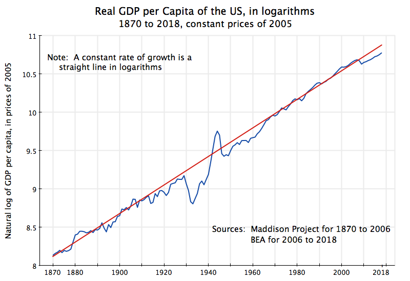
Such an increase in productivity is not outside the norm for the US.  Indeed, it matches what the US has experienced over at least the last century and a half.  The chart at the top of this post shows how GDP per capita has grown since 1870.  The chart is plotted in logarithms, and those of you who remember their high school math will recall that a straight line in such a graph depicts a constant rate of growth.  An earlier version of this chart was originally prepared for a prior post on this blog (where one can find further discussion of its implications), and it has been updated here to reflect GDP growth in recent years (using BEA data, with the earlier data taken from the Maddison Project).

What is remarkable is how steady that rate of growth in GDP per capita has been since 1870.  One straight line fits it extraordinarily well for the entire period, with a growth rate of 1.9% a year (or 1.86% to be more precise).  And while the US is now falling below that long-term trend (since around 2008, from the onset of the economic collapse in the last year of the Bush administration), the deviation of recent years is not that much different from an earlier such deviation between the late 1940s to the mid-1960s.  It remains to be seen whether there will be a similar catch-up to the long-term trend in the coming years.

One might reasonably argue that GDP per capita is not quite productivity, which would be GDP per employee.  Over very long periods of time population and the number of workers in that population will tend to grow at a similar pace, but we could also look at GDP per employee:

This chart is based on BEA data, the agency which issues the official GDP accounts for the US, for both real GDP and the number of employees (in full time equivalent terms, so part-time workers are counted in proportion to the number of hours they work).  The figures unfortunately only go back to 1929, the oldest year for which the BEA has issued estimates.  Note also that the rise in GDP during World War II looks relatively modest here, but that is because measures of “real” GDP (when carefully estimated using standard procedures) can deviate more and more as one goes back in time from the base year for prices (2012 here), coupled with major changes in the structure of production (such as during a major war).  But the BEA figures are the best available.

Once again one finds that the pace of productivity growth was remarkably stable over the period, with a growth rate here of 1.74% a year.  It was lower during the Great Depression years, but then recovered during World War II, and was then above the 1929 to 2018 trend from the early 1950s to 1980.  And the same straight line (meaning a constant growth rate) then fit extremely well from 1980 to 2010.

Since 2010 the growth in labor productivity has been more modest, averaging just 0.5% a year from 2010 to 2018.  An important question going forward is whether the path will return to the previous trend.  If it does, the implication is that there will be more job turnover for at least a temporary period.  If it does not, and productivity growth does not return to the path it has been on since 1929, the US as a whole will not be able to enjoy the growth in overall living standards the economy had made possible before.

The McKinsey numbers for what productivity growth might be going forward, of possibly 1.9% a year, are therefore not out of line with what the economy has actually experienced over the years.  It matches the pace as measured by GDP per capita, and while the 1.74% a year found for the last almost 90 years for the measure based on GDP per employee is a bit less, they are close.  And keep in mind that the McKinsey estimate (of 1.9% growth in productivity over 14 years) is of what might be possible, with a broad range of uncertainty over what will actually happen.

The estimate that “about” a quarter of jobs may be displaced by 2030 is therefore not out of line with what the US has experienced for perhaps a century and a half.  Such disruption is certainly still significant, and should be met with measures to assist workers to transition from jobs that have been automated away to the jobs then in need of more workers.  We have not, as a country, managed this very well in the past.  But the challenge is not new.

What will those new jobs be?  While there are needs that are clear to anyone now (as Bernie Sanders noted, which I will discuss below), most of the new jobs will likely be in fields that do not even exist right now.  A careful study by Daron Acemoglu (of MIT) and Pascual Restrepo (of Boston University), published in the American Economic Review in 2018, found that about 60% of the growth in net new jobs in the US between 1980 and 2015 (an increase of 52 million, from 90 million in 1980 to 142 million in 2015) were in occupations where the specific title of the job (as defined in surveys carried out by the Census Bureau) did not even exist in 1980.  And there was a similar share of those with new job titles over the shorter periods of 1990 to 2015 or 2000 to 2015.  There is no reason not to expect this to continue going forward.  Most new jobs are likely to be in positions that are not even defined at this point.

C.  What Would the Candidates Do?

I will not comment on all the answers provided by the candidates (some of which were indecipherable), but just a few.

Bernie Sanders provided perhaps the best response by saying there is much that needs to be done, requiring millions of workers, and if government were to proceed with the programs needed, there would be plenty of jobs.  He cited specifically the need to rebuild our infrastructure (which he rightly noted is collapsing, and where I would add is an embarrassment to anyone who has seen the infrastructure in other developed economies).  He said 15 million workers would be required for that.  He also cited the Green New Deal (requiring 20 million workers), as well as needs for childcare, for education, for medicine, and in other areas.

There certainly are such needs.  Whether we can organize and pay for such programs is of course critical and would need to be addressed.  But if they can be, there will certainly be millions of workers required.

Sanders was also asked by the moderator specifically about his federal jobs guarantee proposal (and indeed the jobs topic was introduced this way).  But such a policy proposal is more problematic, and separate from the issue of whether the economy will need so many workers.  It is not clear how such a jobs guarantee, provided by the federal government, would work.  The Sanders campaign website provides almost no detail.  But a number of questions need to be addressed.  To start, would such a program be viewed as a temporary backstop for a worker, to be used when he or she cannot find another reasonable job at a wage they would accept, or something permanent?  If permanent, one is really talking more of an expanded public sector, and that does not seem to be the intention of a jobs guarantee program.  But if a backstop, how would the wage be set?  If too high, no workers would want to leave and take a different job, and the program would not be a backstop.  And would all workers in such a program be paid the same, or different based on their skills?  Presumably one would pay an engineer working on the design of infrastructure projects more than someone with just a high school degree.  But how would these be determined?  Also, with a job guarantee, can someone be fired?  Suppose they often do not show up for work?

So there are a number of issues to address, and the answers are not clear.  But more fundamentally, if there is not a shortage of jobs but rather of workers (keep in mind that the unemployment rate is now at a 50 year low), why does one need such a guarantee?  It might be warranted (on a temporary basis) during an economic downturn, when unemployment is high, but why now, when unemployment is low?  [October 28 update:  The initial version of this post had an additional statement here saying that the federal government already had “something close to a job guarantee”, as you could always join the Army.  However, as a reader pointed out, while that once may have been true, it no longer is.  So that sentence has been deleted.]

Andrew Yang responded next, arguing for his proposal of a universal basic income that would provide every adult in the country with a grant of $1,000 per month, no questions asked.  There are many issues with such a proposal, which I will address in a subsequent blog post, but would note here that his basic argument for such a universal grant follows from his assertion that jobs will be scarce due to automation.  He repeatedly asserted in the debate that we have now entered into what has been referred to as the “Fourth Industrial Revolution”, where automation will take over most jobs and millions will be forced out of work.

But as noted above, what we have seen in the US over the last 150 years (at least) is not that much different from what is now forecast for the next few decades.  Automation will reduce the number of workers needed to produce some given amount, and productivity per worker will rise.  And while this will be disruptive and lead to a good deal of job displacement (important issues that certainly need to be addressed), the pace of this in the coming decades is not anticipated to be much different from what the country has seen over the last 150 years.

A universal basic income is fundamentally a program of redistribution, and given the high and growing degree of inequality in the US, a program of redistribution might well be warranted.  I will discuss this is a separate blog post.  But such a program is not needed to provide income to workers who will be losing jobs to automation, as there will be jobs if we follow the right macro policies.  And $12,000 a year would not nearly compensate for a lost job anyway.

Elizabeth Warren’s response to the jobs question was different.  She argued that jobs have been lost not due to automation, but due to poor international trade policies.  She said:  “the data show that we have had a lot of problems with losing jobs, but the principal reason has been bad trade policy.”

Actually, this is simply not true, and the data do not support it.  There have been careful studies of the issue, but it is easy enough to see in the numbers.  For example, in an earlier post on this blog from 2016, I examined what the impact would have been on the motor vehicle sector if the US had moved to zero net imports in the sector (i.e. limiting car imports to what the US exports, which is not very much).  Employment in the sector would then have been flat, rather than decline by 17%, between the years 1967 and 2014.  But this impact would have been dwarfed by the impact of productivity gains.  The output of the motor vehicle (in real terms) was 4.5 times higher in 2014 than what it was in 1967.  If productivity had not grown, they would then have required 4.5 times as many workers.  But productivity did grow – by 5.4 times.  Hence the number of workers needed to produce the higher output actually went down by the 17% observed.  Banning imports would have had almost no effect relative to this.

D.  Summary and Conclusion

Automation is important, but is nothing new.  The Luddites destroyed factory machinery in the early 1800s in England due to a belief that the machines were taking away their jobs and that they would then be left with no prospects.  And data for the US that goes back to at least 1870 shows such job “destroying” processes have long been underway.  They have not accelerated now.  Indeed, over the past decade the pace has slowed (i.e. less job “destruction”).  But it is too soon to tell whether this deceleration is similar to fluctuations seen in the past, where there were occasional deviations but then always a return to the long-term path.

Looking forward, careful studies such as those carried out by McKinsey have estimated how many jobs may be exposed to automation (using technologies that we know already to be technically feasible).  While they emphasize that any such forecasts are subject to a great deal of uncertainty, McKinsey’s midpoint scenario estimates that perhaps 23% of jobs may be substituted away by automation between 2016 and 2030.  If so, such a pace (of 1.9% a year) would be similar to what productivity growth has been historically in the US.  There is nothing new here.

But while nothing new, that does not mean it should be ignored.  It will lead, just as it has in the past, to job displacement and disruption.  There is plenty of scope for government to assist workers in finding appropriate new jobs, and in obtaining training for them, but the US has historically never done this all that well.  Countries such as Germany have been far better at addressing such needs.

The candidate responses did not, however, address this (other than Andrew Yang saying government supported training programs in the US have not been effective).  While Bernie Sanders correctly noted there is no shortage of needs for which workers will be required, he has also proposed a jobs guarantee to be provided by the federal government.  Such a guarantee would be more problematic, with many questions not yet answered.  But it is also not clear why it would be needed in current circumstances anyway (with an economy at full employment).

Andrew Yang argued the opposite:  That the economy is facing a structural problem that will lead to mass unemployment due to automation, with a Fourth Industrial Revolution now underway that is unprecedented in US history.  But the figures show this not to be the case, with forecast prospects similar to what the US has faced in the past.  Thus the basis for his argument that we now need to do something fundamentally different (a universal basic income of $1,000 a month for every adult) falls away.  And I will address the $1,000 a month itself in a separate blog post.

Finally, Elizabeth Warren asserted that the problem stems primarily from poor international trade policy.  If we just had better trade policy, she said, there would be no jobs problem.  But this is also not borne out by the data.  Increased imports, even in the motor vehicle sector (which has long been viewed as one of the most exposed sectors to international trade), explains only a small fraction of why there are fewer workers needed in that sector now than was the case 50 years ago.  By far the more important reason is that workers in the sector are now far more productive.

The Economy Under Trump in 8 Charts – Mostly as Under Obama, Except Now With a Sharp Rise in the Government Deficit

A.  Introduction

President Trump is repeatedly asserting that the economy under his presidency (in contrast to that of his predecessor) is booming, with economic growth and jobs numbers that are unprecedented, and all a sign of his superb management skills.  The economy is indeed doing well, from a short-term perspective.  Growth has been good and unemployment is low.  But this is just a continuation of the trends that had been underway for most of Obama’s two terms in office (subsequent to his initial stabilization of an economy, that was in freefall as he entered office).

However, and importantly, the recent growth and jobs numbers are only being achieved with a high and rising fiscal deficit.  Federal government spending is now growing (in contrast to sharp cuts between 2010 and 2014, after which it was kept largely flat until mid-2017), while taxes (especially for the rich and for corporations) have been cut.  This has led to standard Keynesian stimulus, helping to keep growth up, but at precisely the wrong time.  Such stimulus was needed between 2010 and 2014, when unemployment was still high and declining only slowly.  Imagine what could have been done then to re-build our infrastructure, employing workers (and equipment) that were instead idle.

But now, with the economy at full employment, such policy instead has to be met with the Fed raising interest rates.  And with rising government expenditures and falling tax revenues, the result has been a rise in the fiscal deficit to a level that is unprecedented for the US at a time when the country is not at war and the economy is at or close to full employment.  One sees the impact especially clearly in the amounts the US Treasury has to borrow on the market to cover the deficit.  It has soared in 2018.

This blog post will look at these developments, tracing developments from 2008 (the year before Obama took office) to what the most recent data allow.  With this context, one can see what has been special, or not, under Trump.

First a note on sources:  Figures on real GDP, on foreign trade, and on government expenditures, are from the National Income and Product Accounts (NIPA) produced by the Bureau of Economic Analysis (BEA) of the Department of Commerce.  Figures on employment and unemployment are from the Bureau of Labor Statistics (BLS) of the Department of Labor.  Figures on the federal budget deficit are from the Congressional Budget Office (CBO).  And figures on government borrowing are from the US Treasury.

B.  The Growth in GDP and in the Number Employed, and the Unemployment Rate

First, what has happened to overall output, and to jobs?  The chart at the top of this post shows the growth of real GDP, presented in terms of growth over the same period one year before (in order to even out the normal quarterly fluctuations).  GDP was collapsing when Obama took office in January 2009.  He was then able to turn this around quickly, with positive quarterly growth returning in mid-2009, and by mid-2010 GDP was growing at a pace of over 3% (in terms of growth over the year-earlier period).  It then fluctuated within a range from about 1% to almost 4% for the remainder of his term in office.  It would have been higher had the Republican Congress not forced cuts in fiscal expenditures despite the continued unemployment.  But growth still averaged 2.2% per annum in real terms from mid-2009 to end-2016, despite those cuts.

GDP growth under Trump hit 3.0% (over the same period one year before) in the third quarter of 2018.  This is good.  And it is the best such growth since … 2015.  That is not really so special.

Net job growth has followed the same basic path as GDP:


Jobs were collapsing when Obama took office, he was quickly able to stabilize this with the stimulus package and other measures (especially by the Fed), and job growth resumed.  By late 2011, net job growth (in terms of rolling 12-month totals (which is the same as the increase over what jobs were one year before) was over 2 million per year.  It went to as high as 3 million by early 2015.  Under Trump, it hit 2 1/2 million by September 2018.  This is pretty good, especially with the economy now at or close to full employment.  And it is the best since … January 2017, the month Obama left office.

Finally, the unemployment rate:

Unemployment was rising rapidly as Obama was inaugurated, and hit 10% in late 2009.  It then fell, and at a remarkably steady pace.  It could have fallen faster had government spending not been cut back, but nonetheless it was falling.  And this has continued under Trump.  While commendable, it is not a miracle.

C.  Foreign Trade

Trump has also launched a trade war.  Starting in late 2017, high tariffs were imposed on imports of certain foreign-produced products, with such tariffs then raised and extended to other products when foreign countries responded (as one would expect) with tariffs of their own on selected US products.  Trump claims his new tariffs will reduce the US trade deficit.  As discussed in an earlier blog post, such a belief reflects a fundamental misunderstanding of how the trade balance is determined.

But what do we see in the data?:

The trade deficit has not been reduced – it has grown in 2018.  While it might appear there had been some recovery (reduction in the deficit) in the second quarter of the year, this was due to special factors.  Exports primarily of soybeans and corn to China (but also other products, and to other countries where new tariffs were anticipated) were rushed out in that quarter in order arrive before retaliatory tariffs were imposed (which they were – in July 2018 in the case of China).  But this was simply a bringing forward of products that, under normal conditions, would have been exported later.  And as one sees, the trade balance returned to its previous path in the third quarter.

The growing trade imbalance is a concern.  For 2018, it is on course for reaching 5% of GDP (when measured in constant prices of 2012).  But as was discussed in the earlier blog post on the determination of the trade balance, it is not tariffs which determine what that overall balance will be for the economy.  Rather, it is basic macro factors (the balance between domestic savings and domestic investment) that determine what the overall trade balance will be.  Tariffs may affect the pattern of trade (shifting imports and exports from one country to another), but they won’t reduce the overall deficit unless the domestic savings/investment balance is changed.  And tariffs have little effect on that balance.

And while the trend of a growing trade imbalance since Trump took office is a continuation of the trend seen in the years before, when Obama was president, there is a key difference.  Under Obama, the trade deficit did increase (become more negative), especially from its lowest point in the middle of 2009.  But this increase in the deficit was not driven by higher government spending – government spending on goods and services (both as a share of GDP and in constant dollar terms) actually fell.  That is, government savings rose (dissavings was reduced, as there was a deficit).  Private domestic savings was also largely unchanged (as a share of GDP).  Rather, what drove the higher trade deficit during Obama’s term was the recovery in private investment from the low point it had reached in the 2008/09 recession.

The situation under Trump is different.  Government spending is now growing, as is the government deficit, and this is driving the trade deficit higher.  We will discuss this next.

D.  Government Accounts

An increase in government spending is needed in an economic downturn to sustain demand so that unemployment will be reduced (or at least not rise by as much otherwise).  Thus government spending was allowed to rise in 2008, in the last year of the Bush administration, in response to the downturn that began in December 2007.  This continued, and was indeed accelerated, as part of the stimulus program passed by Congress soon after Obama took office.  But federal government spending on goods and services peaked in mid-2010, and after that fell.  The Republican Congress forced further expenditure cuts, and by late 2013 the federal government was spending less (in real terms) than it was in early 2008:

This was foolish.  Unemployment was over 9 1/2% in mid-2010, and still over 6 1/2% in late-2013 (see the chart of the unemployment rate above).  And while the unemployment rate did fall over this period, there was justified criticism that the pace of recovery was slow.  The cuts in government spending during this period acted as a major drag on the economy, holding back the pace of recovery.  Never before had a US administration done this in the period after a downturn (at least not in the last half-century where I have examined the data).  Government spending grew especially rapidly under Reagan following the 1981/82 downturn.

Federal government spending on goods and services was then essentially flat in real terms from late 2013 to the end of Obama’s term in office.  And this more or less continued through FY2017 (the last budget of Obama), i.e. through the third quarter of CY2018.  But then, in the fourth quarter of CY2017 (the first quarter of FY2018, as the fiscal year runs from October to September), in the first full budget under Trump, federal government spending started to rise sharply.  See the chart above.  And this has continued.

There are certainly high priority government spending needs.  But the sequencing has been terribly mismanaged.  Higher government spending (e.g. to repair our public infrastructure) could have been carried out when unemployment was still high.  Utilizing idle resources, one would not only have put people to work, but also would have done this at little cost to the overall economy.  The workers were unemployed otherwise.

But higher government spending now, when unemployment is low, means that workers hired for government-funded projects have to be drawn from other activities.  While the unemployment rate can be squeezed downward some, and has been, there is a limit to how far this can go.  And since we are close to that limit, the Fed is raising interest rates in order to curtail other spending.

One sees this in the numbers.  Overall private fixed investment fell at an annual rate of 0.3% in the third quarter of 2018 (based on the initial estimates released by the BEA in late October), led by a 7.9% fall in business investment in structures (offices, etc.) and by a 4.0% fall in residential investment (homes).  While these are figures only for one quarter (there was a deceleration in the second quarter, but not an absolute fall), and can be expected to eventually change (with the economy growing, investment will at some point need to rise to catch up), the direction so far is worrisome.

And note also that this fall in the pace of investment has happened despite the huge cuts in corporate taxes from the start of this year.  Trump officials and Republicans in Congress asserted that the cuts in taxes on corporate profits would lead to a surge in investment.  Many economists (including myself, in the post cited above) noted that there was little reason to believe such tax cuts would sput corporate investment.  Such investment in the US is not now constrained by a lack of available cash to the corporations, so giving them more cash is not going to make much of a difference.  Rather, that windfall would instead lead corporations to increase dividends as well as share buybacks in order to distribute the excess cash to their shareholders.  And that is indeed what has happened, with share buybacks hitting record levels this year.

Returning to government spending, for the overall impact on the economy one should also examine such spending at the state and local level, in addition to the federal.  The picture is largely similar:

This mostly follows the same pattern as seen above for federal government spending on goods and services, with the exception that there was an increase in total government spending from early 2014 to early-2016, when federal spending was largely flat.  This may explain, in part, the relatively better growth in GDP seen over that period (see the chart at the top of this post), and then the slower pace in 2016 as all spending leveled off.

But then, starting in late-2017, total government expenditures on goods and services started to rise.  It was, however, largely driven by the federal government component.  Even though federal government spending accounted only for a bit over one-third (38%) of total government spending on goods and services in the quarter when Trump took office, almost two-thirds (65%) of the increase in government spending since then was due to higher spending by the federal government.  All this is classical Keynesian stimulus, but at a time when the economy is close to full employment.

So far we have focused on government spending on goods and services, as that is the component of government spending which enters directly as a component of GDP spending.  It is also the component of the government accounts which will in general have the largest multiplier effect on GDP.  But to arrive at the overall fiscal deficit, one must also take into account government spending on transfers (such as for Social Security), as well as tax revenues.  For these, and for the overall deficit, it is best to move to fiscal year numbers, where the Congressional Budget Office (CBO) provides the most easily accessible and up-to-date figures.

Tracing the overall federal fiscal deficit, now by fiscal year and in nominal dollar terms, one finds:

The deficit is now growing (the fiscal balance is becoming more negative) and indeed has been since FY2016.  What happened in FY2016?  Primarily there was a sharp reduction in the pace of tax revenues being collected.  And this has continued through FY2018, spurred further by the major tax cut bill of December 2017.  Taxes had been rising, along with the economic recovery, increasing by an average of $217 billion per year between FY2010 and FY2015 (calculated from CBO figures), but this then decelerated to a pace of just $26 billion per year between FY2015 and FY2018, and just $13 billion in FY2018.  The rate of growth in taxes between FY2015 and FY2018 was just 0.8%, or less even than just inflation.

Federal government spending, including on transfers, also rose over this period, but by less than taxes fell.  Overall federal government spending rose by an average of just $46 billion per year between FY2010 and FY2015 (a rate of growth of 1.3% per annum, or less than inflation in those years), and then by $140 billion per year (in nominal dollar terms) between FY2015 and FY2018.  But this step up in overall spending (of $94 billion per year) was well less than the step down in the pace of tax collection (a reduction of $191 billion per year, the difference between $217 billion annual growth over FY2010-15 and the $26 billion annual growth over FY2015-18).

That is, about two-thirds (67%) of the increase in the fiscal deficit since FY2015 can be attributed to taxes being cut, and just one-third (33%) to spending going up.

Looking forward, this is expected to get far worse.  As was discussed in an earlier post on this blog, the CBO is forecasting (in their most recent forecast, from April 2018) that the fiscal deficits under Trump will reach close to $1 trillion in FY2019, and will exceed 5% of GDP for most of the 2020s.  This is unprecedented for the US economy at full employment, other than during World War II.  Furthermore, these CBO forecasts are under the optimistic scenario that there will be no economic downturn over this period.  But that has never happened before in the US.

Deficits need to be funded by borrowing.  And one sees an especially sharp jump in the net amount being borrowed in the markets in CY 2018:


These figures are for calendar years, and the number for 2018 includes what the US Treasury announced on October 29 it expects to borrow in the fourth quarter.  Note this borrowing is what the Treasury does in the regular, commercial, markets, and is a net figure (i.e. new borrowing less repayment of debt coming due).  It comes after whatever the net impact of public trust fund operations (such as for the Social Security Trust Fund) is on Treasury funding needs.

The turnaround in 2018 is stark.  The US Treasury now expects to borrow in the financial markets, net, a total of $1,338 billion in 2018, up from $546 billion in 2017.  And this is at time of low unemployment, in sharp contrast to 2008 to 2010, when the economy had fallen into the worst economic downturn since the Great Depression  Tax revenues were then low (incomes were low) while spending needed to be kept up.  The last time unemployment was low and similar to what it is now, in the late-1990s during the Clinton administration, the fiscal accounts were in surplus.  They are far from that now. 

E. Conclusion 

The economy has continued to grow since Trump took office, with GDP and employment rising and unemployment falling.  This has been at rates much the same as we saw under Obama.  There is, however, one big difference.  Fiscal deficits are now rising rapidly.  Such deficits are unprecedented for the US at a time when unemployment is low.  And the deficits have led to a sharp jump in Treasury borrowing needs.

These deficits are forecast to get worse in the coming years even if the economy should remain at full employment.  Yet there will eventually be a downturn.  There always has been.  And when that happens, deficits will jump even further, as taxes will fall in a downturn while spending needs will rise.

Other countries have tried such populist economic policies as Trump is now following, when despite high fiscal deficits at a time of full employment, taxes are cut while government spending is raised.  They have always, in the end, led to disasters.