
Chart 1
A. Introduction
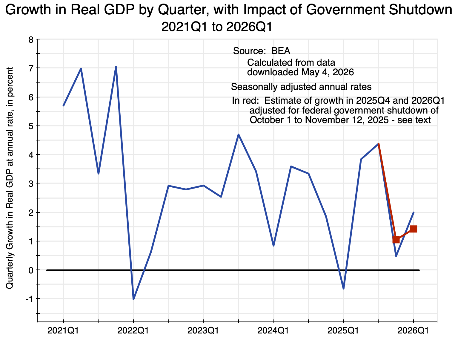
The Bureau of Economic Analysis of the US Department of Commerce (BEA) released on April 30 its initial estimate (what it calls its “Advance Estimate”) of the GDP accounts for the first quarter of 2026. The headline rate was of growth in real GDP in the quarter of 2.0% (at an annual rate). While it noted that this was due in part to a rise in government spending in the first quarter relative to the fourth of 2025 (as government spending recovered from a temporarily depressed level due to the federal government shutdown in October/November), the way this impacted GDP may not be clear to many. The impact being referred to was not due to a demand effect, as some might assume and as may seem to be implied by the use of the word “spending”. Rather, it was a supply-side effect – a consequence of how the government’s direct contribution to the nation’s output is measured in the standard GDP accounts
The way the government’s contribution is measured in the GDP accounts (which are more properly referred to as the National Income and Product Accounts, or NIPA) and the contrast with how production is measured in the private sector accounts, is of interest as it goes to the basic concepts of what GDP is and how it is measured and estimated. One purpose of this post is to review those basic concepts, and contrast how the value of private production is estimated versus how the value of government-provided services is estimated.
The measure of the impact of the government shutdown also brings out that viewing GDP as a total demand for goods and services (for private consumption, investment, government spending, and net exports) can be misleading. GDP is in fact a measure of production (GDP = Gross Domestic Product), and that production is equal to what is counted in demand only due to the fact that investment includes changes in inventories. If the total supplied (of an individual product as well as all products together) exceeds the demand for it, then the excess is accumulated as an increase in inventories – and an increase in inventories is an investment. That investment in higher inventories is counted along with other investments, and for this reason we can estimate how much was produced (GDP) based on the demands. And if total demand exceeds total supply then inventories are drawn down, leading to negative investment in inventories.
I should hasten to add that this does not imply that the demand side components of GDP are unimportant. They are extremely important, as production in a modern economy is primarily driven by demand (up to capacity constraints). It is just that the demand side and the supply side are different. They should not be confused, and they often are.
While government spending on goods and services is, indeed, an important component of total (or aggregate) demand, what is often lost in the discussion is that government also provides services itself. This is a direct contribution to GDP, and while the BEA provides a measure of it, few people pay much attention to it. The BEA has to approach this estimation of the provision of government-produced services differently, however, than how it estimates the value of private goods and services produced. The issue is that while private goods and services are sold at some price – with their value measured by that price – government services are not sold but are rather provided without charge. The issue then is how to estimate the value of these government services.
Section B of this post will first review how the value of private goods and services produced – their contribution to GDP – is measured in the GDP accounts. The section following that will then review how this is done for the government provision of services, with its contribution to GDP. The section will also look more broadly at how the BEA arrives at its estimate of government expenditures as a demand item in the GDP accounts – the government spending concept that people focus on when considering GDP.
The penultimate section will then apply this to estimate the direct impact on GDP of the federal government shutdown that took place from October 1 to November 12, 2025, with a resulting impact on GDP in the fourth quarter of 2025. We find that the direct impact of the shutdown was that the growth rate of GDP in the fourth quarter of 2025 would have been 0.6% point higher (0.57% higher to be more precise), i.e. growth would have been at a rate of 1.1% rather than the 0.5% estimated. And then, had there been no shutdown, growth in the first quarter of 2026 would have been 0.6% point lower (as it would be starting from a 0.6% higher base), i.e. growth of 1.4% rather than the 2.0% announced.
These growth rates in the absence of a federal government shutdown – of 1.1% in the fourth quarter and 1.4% in the first quarter – are shown in red in the chart at the top of this post. The growth rates are not high, but they tell a different story than what one might conclude from the unadjusted figures. Instead of low growth at the end of 2025 with a significant bounce back in early 2026, growth was middling throughout. But as seen in the chart at the top of this post, the growth – while on the low side – was within the range seen in recent years.
I should also emphasize that this measure of the impact of the government shutdown takes into account only the direct effects of the shutdown on the supply of production (i.e. on the supply of government services). It does not attempt to measure what the indirect impacts might have been. The BEA is referring to this direct impact in the brief notes it attached to its news releases of the GDP accounts for the fourth quarter of 2025.
The BEA provided a somewhat different estimate than the one obtained here of the direct impact of the government shutdown, saying that it reduced GDP growth by “about 1.0 percentage point” in the fourth quarter of 2025. The reason for that discrepancy with the 0.57% point estimate calculated here is not clear. And while each of the three releases of its estimates of GDP in the fourth quarter of 2025 (i.e. the Advance, Second, and Third Estimates) uses the same language and the same estimate of a 1.0% point reduction, the recent news release for the first quarter off 2026 failed to say that in the absence of the shutdown, GDP growth in the first quarter of 2026 was 1.0% point higher than it otherwise would have been. That is, in the absence of the shutdown (which depressed GDP in the fourth quarter of 2025), growth in the first quarter of 2026 would have been 1.0% (at an annual rate) rather than the 2.0% reported.
The 1.0% point estimate for the direct impact of the shutdown is higher than the 0.6% estimate made here. The reason for this difference is not clear. A guess at why this is the case will be discussed in the concluding section of this post.
B. The Measurement of the Contribution to GDP from Private Production
Previous posts on this blog (see here and here, for example) have discussed that GDP is estimated by the BEA in three separate ways. The BEA discusses this in more detail in Chapter 2: Fundamental Concepts, of its NIPA (National Income and Product Accounts) Handbook. The three approaches should each lead to the same estimate of GDP. In practice there will be differences due to statistical noise and other such issues, but the three approaches serve as a good check on each other. They also provide for a better understanding of what GDP means as a concept.
The first – and most commonly discussed – approach estimates GDP from the demand side, by adding up estimates of how production is used (for private consumption, private investment, government consumption and investment, and exports net of imports). As discussed above, with additions to inventories counted as an investment, this total will match the total supply of what is produced. It is also the basis of the first estimate of GDP that the BEA releases, which comes out normally about one month after the end of each quarter in its release of the “Advance Estimate” of the GDP accounts.
A second method is to estimate the incomes generated. Whatever is produced leads to income for someone – wages of labor and profits of the owners and investors – so total incomes should match GDP. To reduce confusion, the BEA labels this estimate Gross Domestic Income (GDI). In principle it should be the same as GDP and will differ only because these are all statistical estimates. The BEA normally releases its first estimate of GDI about two months after the end of each quarter, with it included (along with updated estimates of GDP) in its “Second Estimate” of the GDP accounts.
The third method is to estimate the value created in each sector of production. Aggregated across sectors, that value should also match GDP. To avoid double-counting, the estimates are of the value that is added in each sector (i.e. the value created on top of the intermediate inputs used that were obtained from other sectors). The BEA refers to this as the value added in each sector. The total across the economy is Gross Value Added. This Gross Value Added should also match the estimates of GDP (from the demand side) and GDI (from the income side), although there will be differences in the estimates themselves due to statistical issues. The BEA normally releases its first estimate of value added by sector about three months after the end of each quarter, with it included (along with updated estimates of GDP and GDI) in its “Third Estimate” of the GDP accounts.
What is of interest to us here is how the BEA arrives at this third estimate of GDP, i.e. of value added by sector. Based on monthly sample surveys of firms (and later updated by more comprehensive annual surveys and ultimately by censuses of firms undertaken every five years), the BEA obtains information at the firm level of what its total sales were, how much was spent on intermediate inputs, what was paid in wages and other compensation to its workers, and what then remained as profits. This is in broad terms: there will be more detail in what is gathered, but the basic categories are what are of interest to us here. Note also that these are all measured in nominal terms, i.e. in terms of dollars spent and received.
From this, the BEA can determine for its sample of firms (selected to provide representative samples of each sector) what their gross production was during the period (equal to what was sold as adjusted for inventories) and the value of the intermediate inputs purchased. The difference is the value added. Part of that value added then goes to wages and other compensation for labor. What then remains (after certain indirect taxes) is operating profit. The profits are generated in part by the capital invested in the firm, and that capital will be used up over time – i.e. it depreciates. Hence part of the profit is allocated (at least notionally) to cover an allowance for depreciation, and what remains after that allowance is termed the “net operating surplus”. The net operating surplus will then be made up of what is paid in interest and in rents, and then in the remaining profits of firms (whether incorporated or unincorporated).
As noted above, all these estimates are in current dollar terms, with the value added of the firms obtained by subtracting the purchases of intermediate inputs from gross production. But we also want to see what the changes over time were in real terms – i.e. adjusted for price changes. For this, the BEA estimates separately average price increases for each sector, drawing on a range of separate data sources – many from the Bureau of Labor Statistics (BLS). These do not come from the firm-level surveys, but rather from separate surveys of changes in prices for standard goods and services of a given quality.
The estimation of value added by sector for private producers is therefore conceptually straightforward. There will of course be challenges in its implementation, but one can start with the values of what is produced in each sector. Those values are known because the goods and services are sold on a market, and GDP is a measure of the market values of what was produced. (Some have argued that market values are not a good measure of the “true” value of what the economy produces. But the question then is what value to use? How does one value a glass of drinking water, for example? It is of enormous value to someone dying of thirst, and presumably of greater value to any individual than whatever they paid for it, but how much greater? There is no way to know this. Hence market values are used, i.e. what was paid for it. But this is a separate debate.)
Sales on the market can thus provide a measure that can be used to determine the value (the market value) of what private firms produce, with GDP derived from and based on this. But what to do when services are provided by government entities? Those services are not sold in a market, but rather are provided without charge. That will be addressed in the next section.
C. The Measurement of the Contribution to GDP from Government Production
When government is discussed in relation to the NIPA accounts, the focus is almost always on government demand as one of the basic demand components of GDP (along with private consumption, private investment, and exports less imports). The government’s role as a source of aggregate demand is certainly important. In an economic downturn, an increase in government expenditures can and has played a critical role in returning the economy to growth and thus generating employment. The contrasting experiences following the 2008 economic and financial collapse (with the later slow recovery, as the Republican-controlled Congress forced through government expenditure cuts) and that following the Covid crisis of 2020 (where massive government expenditures – in both 2020 under Trump and in 2021 under Biden – led to a quick recovery to full employment) are clear examples.
Keynes was right, and hopefully he will not once again be forgotten. But as important as that is, there is more to government in the NIPA accounts that is often overlooked. There is in particular a direct role of government on the supply side of the accounts. It is in the government’s role as a supplier of services that there was a direct impact on GDP in the fourth quarter of 2025 as a result of the federal government shutdown.
Governments produce services. Those services are valuable, and contribute to a nation’s well-being. At the state and local level, those services will include the services of public school teachers, police officers, fire and other first responders, and others. At the federal level, the services include those of the scientists who work at the weather bureau or NASA or the energy research labs; the medical researchers and officials at NIH, the CDC, and the FDA; those who take care of and manage our National Parks and other public resources; and the soldiers in the nation’s armed forces who provide for the common defense. They also include the services of the administrators of programs such as Social Security and Medicare, as well the programs to build and maintain our public highways and other public infrastructure, and much more. Their work is valuable and should be (and is) counted in GDP.
But in general there is no charge (or only a minimal charge) for those services. There are some exceptions, where government entities may charge an amount that may fully cover their costs, but at the federal level there are not many. An example would be the Tennessee Valley Authority, or the Post Office. The accounts for such government enterprises are separated from what are referred to as the “general government” accounts. The “government” figures in the NIPA accounts that are usually referred to are the accounts for general government and exclude government enterprises.
For general government, the question then is how to value the services provided, since no fee (or essentially no fee) is charged for those services. While taxes are paid, those taxes are not linked directly to particular services used. And while there may sometimes be fees for certain services (such as admission fees to national parks, or passport and other such application fees), such fees are modest in the government sector – especially at the federal level.
Given all this, the BEA (and indeed national statistical agencies around the world) estimate the value added from the public services provided based on the cost of providing those services. There are two components to those costs. One is the wages and other compensation paid to government employees. The other is for the depreciation of the capital assets of the public sector. Those capital assets include, for example, roads. There is an initial investment cost to build those roads and over time those roads depreciate.
Comparing this to the estimation of value added in the private sectors of the economy, one can see similarities. As discussed above, the value added generated by private firms (i.e. the value of the gross production minus expenditures on intermediate inputs) will equal the wages and other compensation paid to the labor employed, plus a charge for the depreciation of the capital used in the sector, plus remaining profits after wages and depreciation are subtracted. In the case of the provision of government services, the value added is similar except that there is no charge for remaining profits after wages are paid and depreciation is accounted for. The implicit assumption is that the rate of return on capital after depreciation is zero.
Thus the measure of value added from the provision of government services is built bottom-up from the cost of providing those services (i.e. the wage and depreciation costs). This is in contrast to the top-down calculation in the private sector accounts that starts with the market value of what is produced and ends with a residual amount as after-depreciation profits accruing to the firm. In the government accounts the after-depreciation profits are valued as if they were zero, but the rest is in essence the same.
This estimate of government value added when added to the intermediate purchases by government of goods and services from other sectors, will then equal the gross output of general government. Again, this is similar to the concepts in the private sector accounts, but rather than going top-down (i.e. from gross total output less purchases of intermediates to reach value added), the process for the government accounts is bottom-up (i.e. from adding intermediate purchases to value added to yield gross output).
To provide a sense of the magnitudes and to make this concrete, these are the figures for the federal government accounts as provided by the BEA in its Advance Estimate for the accounts for the first quarter of 2026:
Federal Government NIPA Accounts – Advance Estimate for 2026Q1
| Federal Government, annual rates, $ billions | 2026Q1 |
| Gross output of general federal government | 1,597.0 |
| Value added | 1,037.5 |
| Compensation of general government employees | 617.2 |
| Consumption of general government fixed capital | 420.3 |
| Intermediate goods and services purchased | 559.5 |
| Durable goods | 67.6 |
| Nondurable goods | 66.5 |
| Services | 425.4 |
| Less: Own-account investment | 69.9 |
| Less: Sales to other sectors | 13.4 |
| Equals Federal Consumption Expenditures | 1,513.7 |
| Federal Gross Investment | 473.7 |
| Fed Gov’t Consumption + Gross Investment | 1,987.5 |
Source: Interactive NIPA Accounts, mostly from Table 3.10.5, with Table 3.2 for Federal Gross Investment and Table 1.1.5 for the check on total Federal Consumption and Investment. Downloaded May 4, 2026. As for all of the NIPA accounts, the figures are shown at annualized rates.
Compensation of federal government employees ($617.2 billion at an annual rate) is added to an estimate of depreciation ($420.3 billion at an annual rate, where depreciation is more properly referred to in the accounts as “consumption of fixed capital), to yield value-added from the services the federal government produces and provides to the economy ($1,037.5 billion). Adding in purchases of intermediate goods yields gross output of government ($1,597.0 billion). From this a charge is subtracted for “own-account investment” ($69.9 billion). This is a charge for the compensation that was paid to federal workers for work they did in supervising the building of new public capital, e.g. highways and such. That cost is included in the cost of federal government gross investment ($473.7 billion), which is a few lines down and is removed here to avoid double-counting. Also subtracted is a small charge ($13.4 billion) for the relatively minor fees that are collected by government for various services (such as admissions to national parks, as noted before). Those fees are counted either in private household consumption expenditures or in the expenditures of businesses, depending on who pays them.
Federal government gross output ($1,597.0 billion) less the charge for own-account investment ($69.9 billion) and less the charge for sales to other sectors ($13.4 billion) will then yield federal government consumption expenditures ($1,513.7 billion). Adding in federal government gross investment ($473.7 billion, which as noted above includes the cost of federal workers who managed such investment), yields total federal government consumption and investment expenditures of $1,987.5 billion. It is this final figure that is the government expenditures figure found in the demand components of GDP that discussion almost always focuses on.
These federal government expenditures are for goods and services that it either produces itself (the $1.0 trillion of value added) or has purchased from other sectors (whether as intermediates used in government consumption or for investment – close to $1.0 trillion as well). But as some may realize, such expenditures account for only a relatively small share of total federal budget expenditures. There are also transfer payments from the federal government to individuals (about $3.8 trillion at an annual rate currently for programs such as Social Security and Medicare) and to state and local governments ($1.0 trillion). The demands for goods and services arising from those transfers are counted in the NIPA accounts in the accounts for households or for state and local governments. There are also payments of interest on the federal debt ($1.2 trillion) and various other payments, bringing total federal expenditures to $8.5 trillion as of the first quarter of 2026 (at an annual rate). The $1,987.5 billion of federal expenditures on goods and services derived above (the federal government demand component of GDP) are less than one-quarter of that total.
With federal government demand for goods and services close to $2.0 trillion, a bit over half ($1,037.5 billion) comes from value-added produced in the government sector itself. Of this, $617.2 billion reflects the compensation paid to federal government employees. That is, government is a provider of services (that are then treated as being “purchased” by government itself) as well as a purchaser of goods and services from other sectors (of intermediates and for government investment expenditures).
It is government as a producer of services where the federal government shutdown had a direct impact on GDP in the fourth quarter of 2025. The next section of this post will look at how that impact was calculated.
D. The Direct Impact of the Federal Government Shutdown on Government Production
With the federal government shutdown of October 1 to November 12, 2025, most (although not all) federal workers were told to stay home. They were not paid during the shutdown, but based on a law passed in January 2019 (in response to an earlier shutdown), federal workers furloughed during a shutdown are paid following the end of the congressional impasse. (Prior to the January 2019 law approving this for all future shutdowns, Congress had always approved legislation to provide for payment, but passed such legislation each time there was a shutdown.)
The federal government wages and other compensation paid for the period of the shutdown were thus the same as they would have been in the absence of a shutdown. While the payments then came in November (i.e. still within the calendar quarter), all payments in the NIPA accounts are in any case accounted for on an accrual basis – i.e. when the payment obligation is incurred. Thus they are always reflected in the NIPA accounts in the quarter when the shutdown took place, even if the timing was such that the back payments came only later, in a subsequent quarter.
How, then, did the BEA reflect the loss in government produced services as a consequence of the shutdown? It provided a very brief, one paragraph, explanation as a technical note included with its Advance Estimate of 2025Q4 GDP (released on February 20, 2026), and then with the same note in the Second Estimate (released on March 13) and the Third Estimate (released on April 9). It provides a more detailed, one page, explanation on its Frequently Asked Questions page, and an even more complete explanation on the principles followed in estimating the government accounts more generally as Chapter 9 of the NIPA Handbook.
The basic principles are simple. Since the wages will (in the end) be paid to all federal government employees (whether furloughed or not), the total paid in nominal terms is simply the same, regardless of the shutdown. The BEA obtains those figures from the Department of the Treasury. But the BEA then adjusts what the real labor input was based on the proportion that working hours of federal workers were reduced during the quarter, due to some share of the federal workers being placed on furlough. The implicit assumption is that the real provision of government services during the period was reduced in that proportion.
This will then lead to a mechanical increase in the price index in that quarter for the provision of the federal labor services provided, as the price index (in essence a wage index) will equal the compensation paid in nominal terms (unchanged by the shutdown) divided by the real index of labor services provided in the quarter (reduced by the reduction in hours reporting to work in the quarter). That is, the price index for government compensation in the quarter will shoot up, as the ratio of the compensation payments made (unchanged) divided by an index of the hours worked (reduced due to the shutdown) will go up.
The question, then, is what effect the government shutdown had on GDP (and hence its growth) in the quarter. For this, one needs to specify a counterfactual as a basis for comparison. One cannot simply take what the change was in the figure for the real compensation of federal workers in the quarter, as there are always quarter-to-quarter changes in those figures independent of any government shutdown. Also, the price index for government workers changes from one quarter to the next (like for any price index, and generally going up).
But one can specify a reasonable counterfactual from the fact that there was no government shutdown in the first quarter of 2026. Thus the price index for government workers, after shooting up in the figures for the fourth quarter of 2025, will revert to its previous path in the figures published for the first quarter of 2026. We have these. A reasonable assumption to make would be that in the absence of the shutdown, the price index in the fourth quarter of 2025 would have gone up at the same pace as it did over the six-month period from the third quarter of 2025 to the first quarter of 2026 (adjusted, of course, to the quarterly equivalent).
From this, one can calculate what the direct impact was of the government shutdown on the provision of government services and hence on GDP:
Direct Impact of Federal Government Shutdown on GDP
| $ billions or index; annualized change | 2025Q3 | 2025Q4 | Change |
| A) BEA Estimates | |||
| 1) Nominal Gov’t Compensation | $632.5 | $617.2 | -$15.3 |
| 2) Price Index / % Change | 148.779 | 163.688 | 46.5% |
| 3) Real Gov’t Compensation | $425.1 | $377.1 | -$48.0 |
| B) No Gov’t Shutdown Scenario | |||
| 1) Nominal Gov’t Compensation | $632.5 | $617.2 | -$15.3 |
| 2) Price Index / % Change | 148.779 | 150.225 | 3.9% |
| 3) Real Gov’t Compensation | $425.1 | $410.9 | -$14.3 |
| C) Impact on GDP | |||
| 1) Difference in Real Gov’t VA | 0.0 | $33.8 | $33.8 |
| 2) BEA Estimate of GDP | $24,026.8 | $24,055.7 | 0.48% |
| 3) GDP if No Shutdown | $24,026.8 | $24,089.5 | 1.05% |
| Difference in GDP Growth | 0.57% |
Note: “Government” in this table refers to Federal Government only. “Compensation” refers to compensation of federal government employees.
Source: Based on data derived from the Interactive NIPA Accounts. Downloaded May 4, 2026.
Panel A in the table provides the figures directly from the BEA released accounts for the periods (as of April 30, 2026). Nominal compensation of federal workers fell in the fourth quarter – from $632.5 billion in the third quarter to $617.2 billion in the fourth – with this independent of the shutdown. Keep in mind that – as in all of the NIPA accounts – the financial flows are shown at annual rates. The actual flows in any given quarter will be one-fourth of these.
The BEA then estimates that the real input of government labor (based on the number of hours reporting to work, and expressed in terms of 2017 prices) fell from $425.1 billion in the third quarter to $377.1 billion in the fourth. From this, it calculated the implicit price index for this compensation (i.e. the nominal payment divided by the payment in constant 2017 prices), and found that it rose from 148.779 in the third quarter to 163.688 in the fourth.
While the growth rate in the price index looks scary at 46.5%, keep in mind again that the BEA figures (including for growth rates) are all shown in annualized terms in the NIPA accounts. The actual increase in the index in the quarter itself (i.e. from 148.779 to 163.688) is a 10.0% rise. But when compounded as if it were that for a full year (four quarters), the rate is the 46.5% shown.
As noted above, a reasonable counterfactual to estimate the direct impact on GDP from the government shutdown would be to assume the price index for government compensation would have risen in the fourth quarter of 2025 at the same pace as it did between the third quarter of 2025 and the first quarter of 2026 (when it reverted back to its previous path from the special conditions of the fourth quarter). That rate – in annual terms – was just 3.9% – far less than the 46.5% arising due to the shutdown.
Panel B of the table then works out the implications. Nominal federal government wages will be the same. The price index will, however, only rise to 150.225 from the 148.779 of the third quarter (an increase of just under 1.0% – keep in mind that the 3.9% is an annual rate, and is 3.945% to be more precise). The figure for real input of federal workers would thus fall only to $410.9 billion ( = $617.2 / 1.50225) from the $425.1 billion of the third quarter. It still fell, due to the ongoing reductions in the federal labor force, but with no shutdown that fall will be less: a reduction (relative to the third quarter) of $14.3 billion rather than the reduction of $48.0 billion that the BEA estimated with the shutdown (all at annual rates). The difference due to the shutdown is $33.8 billion (in figures before rounding).
GDP in the fourth quarter would thus have been $33.8 billion higher than otherwise. The BEA had estimated that GDP in the fourth quarter was $24,055.7 billion (in terms of constant 2017 prices), an increase of just 0.48% (at an annual rate) from the $24,026.8 billion in the third quarter. Without the direct impact of the shutdown, GDP would have been $33.8 billion higher in the fourth quarter, at $24,089.5 billion. The (annual) growth rate would then have been 1.05%. The difference in the (annual) growth rate was 0.57%, or just under 0.6%.
This impact is significant, although not overwhelming. Growth in the fourth quarter still would have been slow. Indeed, the 0.6% direct impact on growth is less than the change in the BEA’s estimate for GDP growth in the fourth quarter as it gained more data on the quarter. In the Advance Estimate, the BEA estimated GDP in the fourth quarter had grown at a 1.4% annual rate. This was reduced to 0.7% in its Second Estimate and to 0.5% (i.e. rounded from 0.48%) in its Third Estimate. Such changes in the BEA estimates for growth in GDP are not unusual, and the BEA is open about this. But while the BEA receives a substantial amount of additional data on the private sector accounts in the months following its initial set of NIPA estimates, the federal government accounts (which it obtains directly from the Treasury) normally do not change much. Indeed, there were essentially no changes between the three releases in the federal government data used in the table above.
Furthermore, while the direct impact of the shutdown reduced the growth rate of real GDP (as measured) in the fourth quarter by 0.6%, the reversion to the prior path means that the growth in real GDP was a similar 0.6% higher in the first quarter than what it otherwise would have been. That is, to be consistent, one should recognize that while the direct impact of the shutdown would have meant 1.05% growth in the fourth quarter rather than 0.48%, there would then also have been a similar reduction in growth in the first quarter of 2026. This is due to simple arithmetic, as GDP would have started from a higher point in the fourth quarter. The result would have been that instead of 2.0% growth in the first quarter of 2026 (the BEA Advance Estimate), the growth in GDP would have been only 1.4%. Those figures on GDP growth are shown in red in the chart at the top of this post.
E. Concluding Points
The direct impact of the federal government shutdown was small. Furthermore, an honest accounting would recognize that the impact was temporary – any reduction in GDP growth in a given quarter would then be offset (by simple arithmetic) by an increase in GDP growth in the next quarter of a similar amount. But while the Trump White House highlighted the first, it ignored the second.
The BEA calculation of that direct impact has, however, served as a “teachable moment” that can lead to a better understanding of what makes up GDP. While government spending is commonly recognized as an important contributor to GDP demand, many are not aware that government is also a significant contributor to GDP supply. Government workers provide important services, and those services are part of the supply of goods and services that enrich a country. That supply does not come solely from the private sector.
Valuing the supply of services provided by government workers is a challenge. For private production – where goods and services are sold in the market – the statistical agencies producing the national income accounts can use their market values as the basis for the valuation of what is produced. Presumably the true valuation by consumers is even higher, as they will purchase some good or service if their valuation is higher than the price but not if their valuation is lower. But there is no way to know what those consumer valuations are, plus they will be different for each individual as they will depend on that individual’s circumstances.
But government provided services are not sold and thus there is not even that basis for estimating the value of what is produced. The best that can be done is a bottom-up valuation based on the cost of providing those services (i.e. the labor cost and the cost of capital depreciation), where a political process is followed to determine what and how much of such services will be provided. But the top-down valuation that is done for privately produced goods and services is not all that different, once one recognizes how value-added is determined (where GDP is equal to the total of value-added in the economy). The main difference is that while for private production there is a residual profit that accrues to the entity that organized the production, there is no such residual value that can be ascertained for government production. It is implicitly set to zero instead.
The limitations in how the BEA estimated the direct impact on GDP from the shutdown should also be recognized. The BEA had little choice other than to assume that there would be a reduction in federal government output in proportion to the reduction in the number of official working hours of federal workers during the quarter. While it’s probably the only assumption it could make for the estimation, it’s not really a good one. I suspect that many (and probably most) of the federal workers put on furlough continued to work while at home, in order to catch up on reports and other tasks, and to prepare for when they would return to the office. Furthermore, once they did return, there would be a period when they would be doing more than the usual in order to catch up. Thus the BEA estimate of the impact on GDP based on the reduction in the number of formal working hours is probably an overestimate.
On the other side, the overall impact on GDP from the shutdown was almost certainly greater than whatever the direct impact was. Government spending was reduced during the period of the shutdown by some amount, and this will have an impact. Certain contractors were also dismissed during this period (including low-paid workers in the cafeterias and as janitors, as well as more highly paid consultants), and the impact of this on GDP will depend on whether they found alternative employment during that period.
But any assessment of the overall impact can only be done by a model of the impacts, and different analysts will have different models. And the BEA does not do models: they are a statistical agency. Thus they provided an estimate of the direct impact – subject, as discussed above, to the limitation that assumptions would still need to be made on what the counterfactual was. They did not try to provide an estimate of the overall impact on GDP.
The BEA estimate of the direct impact of the shutdown – expressed initially in its news release of the Advance Estimate for the fourth quarter of 2025 (on February 20, 2026), and then repeated in its news releases of the Second and Third estimates – was that the direct impact was a reduction in the growth rate of real GDP in the quarter by “about 1.0 percentage point”. This is somewhat higher than the 0.6 percentage point impact calculated in Section D above. A question is why?
I puzzled over this for some time. Any difference in the calculations should have been well less than a difference between an impact on GDP growth of 0.57% point and an impact of 1.0% point. And working backwards, in order to have an impact on growth of 1.0% point, the real compensation of federal government workers during 2025Q4 would have had to increase from $425.1 billion in the third quarter (in 2017 prices, at an annual rate) to $437.2 billion in the fourth, rather than fall to the BEA’s estimate of $377.1 billion. There would have been no reason for such an increase in the absence of a shutdown, especially as nominal spending on compensation for government workers fell from $632.5 billion in the third quarter to $617.2 billion in the fourth. Compensation of federal workers would also then need to fall back to $406.9 billion – BEA’s estimate of real compensation of federal government workers in the first quarter of 2026. This is not plausible.
In the calculations in Section D above – where it was assumed that the price index for compensation of federal workers would have grown at the same rate in the fourth quarter of 2025 as it did between the third quarter of 2025 and the first quarter of 2026 – real compensation of federal government workers would have gone in the absence of a shutdown from $425.1 billion in the third quarter, to $410.9 billion in the fourth quarter. The fall would then have continued to the $406.9 billion BEA figure for the first quarter of 2026. That would be a reasonable path in the absence of a shutdown. A big increase in the fourth quarter in the absence of a shutdown, followed then by a sharp fall, is highly improbable.
Why then did the BEA releases on GDP in the fourth quarter of 2025 (all three) state that the impact of the government shutdown on the growth in GDP was to subtract “about 1.0 percentage point from real GDP growth in the fourth quarter”? I can only speculate; what follows is purely a guess. As the GDP estimates were being prepared, political appointees in the White House and/or in the Department of Commerce may well have asked BEA staff for their estimate of the impact on GDP growth due to the shutdown. Such a request would not be surprising, but professional staff in the BEA would have to respond that they really cannot say what the overall impact might have been. They are statisticians working with data, and all they could estimate would be what the direct impact would be as a consequence of most federal workers being placed on furlough (with the assumption that their real output would be reduced in proportion to the reduction in the formal number of hours at their work sites).
The BEA may then have arrived at an estimate of an impact of about 0.6% points – as per above. This might have been taken as sounding low, so it was suggested to round this to 1%. And then at some point later, some senior person may have made it 1.0%.
This is pure speculation. But it is unusual that the BEA would have provided such an estimate in its news releases for the GDP estimates for the fourth quarter of 2025. And the BEA did not say in the release of its Advance Estimate for GDP in the first quarter of 2026 that its estimated figure on growth in the quarter (of 2.0%) would have been reduced by 1.0% (or 0.6%) in the absence of the federal government shutdown in the prior quarter. Instead, it only included the qualitative remark that there was an increase in federal government nondefense spending, that this was mainly from an increase in federal employee compensation following its reduction in the fourth quarter of 2025, and that this was “impacted” by the shutdown in the fourth quarter. Furthermore, it would be easy to mistakenly misunderstand the increase in federal government nondefense “spending” in the first quarter (relative to the depressed level in the fourth quarter) as a demand-side impact. The use of the word “spending” would imply this. Rather, it was a supply-side effect from the contribution to GDP supply from the services provided by government employees.
But political appointees may be becoming more involved in what the BEA provides. Starting with the April 9 release of the Third Estimate of GDP for the fourth quarter of 2025, the news releases for the GDP estimates no longer include the standard sets of tables that were provided before. Those tables could be easily scanned to see what the important developments were. Instead, the releases now only include links to different tables (not those given before in the news releases) on the BEA website, where more comprehensive data has always been posted and updated with each news release.
They assert, in the paragraph announcing that they are no longer providing those standard tables, that not making those tables available is an “improvement”, reflecting “modernization” and “streamlining”. It is, of course, anything but. It will now be difficult to quickly find the key developments in the quarter. The data tables now being linked to were not designed for this. The data will all be there, but buried with all the other data in the NIPA accounts. Those tables were designed for reference purposes.
It would have been easy and at essentially no cost to have continued to provide the standard tables of the news releases. The computer programs are written, and they are all then posted as PDF files online. But by ending the publication of these tables, analysts will now focus more of their attention on the “spin” the officials provide in the news releases. What they provide can highlight the points that they want to see emphasized.
This is unfortunate, but consistent with an administration that wishes to better control what news is released and how it is interpreted, including on figures produced by the nation’s statistical agencies. These have not been subject to such political interference before.


You must be logged in to post a comment.