“There’s no reason that we should have big trade deficits with virtually every country in the world.”
“We’re like the piggybank that everybody is robbing.”
“the United States has been taken advantage of for decades and decades”
“Last year,… [the US] lost … $817 billion on trade. That’s ridiculous and it’s unacceptable.”
“Well, if they retaliate, they’re making a mistake. Because, you see, we have a tremendous trade imbalance. … we can’t lose”
Statements made by President Trump at the press conference held as he left the G-7 meetings in, Québec, Canada, June 9, 2018.
A. Introduction
President Trump does not understand basic economics. While that is not a surprise, nor something necessarily required or expected of a president, one should expect that a president would appoint advisors who do understand, and who would tell him when he is wrong. Unfortunately, this president has been singularly unwilling to do so. This is dangerous.
Trump is threatening a trade war. Not only by his words at the G-7 meetings and elsewhere, but also by a number of his actions on trade and tariffs in recent months, Trump has made clear that he believes that a trade deficit is a “loss” to the nation, that countries with trade surpluses are somehow robbing those (such as the US) with a deficit, that raising tariffs can and will lead to reductions in trade deficits, and that if others then also raise their tariffs, the US will in the end necessarily “win” simply because the US has a trade deficit to start.
This is confused on many levels. But it does raise the questions of what determines a country’s trade balance; whether a country “loses” if it has a trade deficit; and what is the role of tariffs. This Econ 101 blog post will first look at the simple economics of what determines a nation’s trade deficit (hint: it is not tariffs); will then discuss what tariffs do and where do they indeed matter; and will then consider the role played by foreign investment (into the US) and whether a trade deficit can be considered a “loss” for the nation (a piggybank being robbed).
B. What Determines the Overall Trade Deficit?
Let’s start with a very simple case, where government accounts are aggregated together with the rest of the economy. We will later then separate out government.
The goods and services available in an economy can come either from what is produced domestically (which is GDP, or Gross Domestic Product) or from what is imported. One can call this the supply of product. These goods and services can then be used for immediate consumption, or for investment, or for export. One can call this the demand for product. And since investment includes any net change in inventories, the goods and services made available will always add up to the goods and services used. Supply equals demand.
One can put this in a simple equation:
GDP + Imports = Domestic Consumption + Domestic Investment + Exports
Re-arranging:
(GDP – Domestic Consumption) – Domestic Investment = Exports – Imports
The first component on the left is Domestic Savings (what is produced domestically less what is consumed domestically). And Exports minus Imports is the Trade Balance. Hence one has:
Domestic Savings – Domestic Investment = Trade Balance
As one can see from the way this was derived, this is simply an identity – it always has to hold. And what it says is that the Trade Balance will always be equal to the difference between Domestic Savings and Domestic Investment. If Domestic Savings is less than Domestic Investment, then the Trade Balance (Exports less Imports) will be negative, and there will be a trade deficit. To reduce the trade deficit, one therefore has to either raise Domestic Savings or reduce Domestic Investment. It really is as straightforward as that.
Where this becomes more interesting is in determining how the simple identity is brought about. But here again, this is relatively straightforward in an economy which, like now, is at full employment. Hence GDP is essentially fixed: It cannot immediately rise by either employing more labor (as all the workers who want a job have one), nor by each of those laborers suddenly becoming more productive (as productivity changes only gradually through time by means of either better education or by investment in capital). And GDP is equal to labor employed times the productivity of each of those workers.
In such a situation, with GDP at its full employment level, Domestic Savings can only rise if Domestic Consumption goes down, as Domestic Savings equals GDP minus Domestic Consumption. But households want to consume, and saving more will mean less for consumption. There is a tradeoff.
The only other way to reduce the trade deficit would then be to reduce Domestic Investment. But one generally does not want to reduce investment. One needs investment in order to become more productive, and it is only through higher productivity that incomes can rise.
Reducing the trade deficit, if desirable (and whether it is desirable will be discussed below), will therefore not be easy. There will be tradeoffs. And note that tariffs do not enter directly in anything here. Raising tariffs can only have an impact on the trade balance if they have a significant impact for some reason on either Domestic Savings or Domestic Investment, and tariffs are not a direct factor in either. There may be indirect impacts of tariffs, which will be discussed below, but we will see that the indirect effects actually could act in the direction of increasing, not decreasing, the trade deficit. However, whichever direction they act in, those indirect effects are likely to be small. Tariffs will not have a significant effect on the trade balance.
But first, it is helpful to expand the simple analysis of the above to include Government as a separate set of accounts. In the above we simply had the Domestic sector. We will now divide that into the Domestic Private and the Domestic Public (or Government) sectors. Note that Government includes government spending and revenues at all levels of government (state and local as well as federal). But the government deficit is primarily a federal government issue. State and local government entities are constrained in how much of a deficit they can run over time, and the overall balance they run (whether deficit or surplus) is relatively minor from the perspective of the country as a whole.
It will now also be convenient to write out the equations in symbols rather than words, and we will use:
GDP = Gross Domestic Product
C = Domestic Private Consumption
I = Domestic Private Investment
G = Government Spending (whether for Consumption or for Investment)
X = Exports
M = Imports
T = Taxes net of Transfers
Note that T (Taxes net of Transfers) will be the sum total of all taxes paid by the private sector to government, minus all transfers received by the private sector from government (such as for Social Security or Medicare). I will refer to this as simply net Taxes (T).
The basic balance of goods or services available (supplied) and goods or services used (demanded) will then be:
GDP + M = C + I + G + X
We will then add and subtract net Taxes (T) on the right-hand side:
GDP + M = (C + T) + I + (G – T) + X
Rearranging:
GDP – (C + T) – (G – T) – I = X – M
(GDP – C – T) – I + (T – G) = X – M
Or in (abbreviated) words:
Dom. Priv. Savings – Dom. Priv. Investment + Govt Budget Balance = Trade Balance
Domestic Private Savings (savings by households and private businesses) is equal to what is produced in the economy (GDP), less what is privately consumed (C), less what is paid in net Taxes (T) by the private sector to the public sector. Domestic Private Investment is simply I, and includes investment both by private businesses and by households (primarily in homes). And the Government Budget Balance is equal to what government receives in net Taxes (T), less what Government spends (on either consumption items or on public investment). Note that government spending on transfers (e.g. Social Security) is already accounted for in net Taxes (T).
This equation is very much like what we had before. The overall Trade Balance will equal Domestic Private Savings less Domestic Private Investment plus the Government Budget Balance (which will be negative when a deficit, as has normally been the case except for a few years at the end of the Clinton administration). If desired, one could break down the Government Budget Balance into Public Savings (equal to net Taxes minus government spending on consumption goods and services) less Public Investment (equal to government spending on investment goods and services), to see the parallel with Domestic Private Savings and Domestic Private Investment. The equation would then read that the Trade Balance will equal Domestic Private Savings less Domestic Private Investment, plus Government Savings less Government Investment. But there is no need. The budget deficit, as commonly discussed, includes public spending not only on consumption items but also on investment items.
This is still an identity. The balance will always hold. And it says that to reduce the trade deficit (make it less negative) one has to either increase Domestic Private Savings, or reduce Domestic Private Investment, or increase the Government Budget Balance (i.e. reduce the budget deficit). Raising Domestic Private Savings implies reducing consumption (when the economy is at full employment, as now). Few want this. And as discussed above, a reduction in investment is not desirable as investment is needed to increase productivity over time.
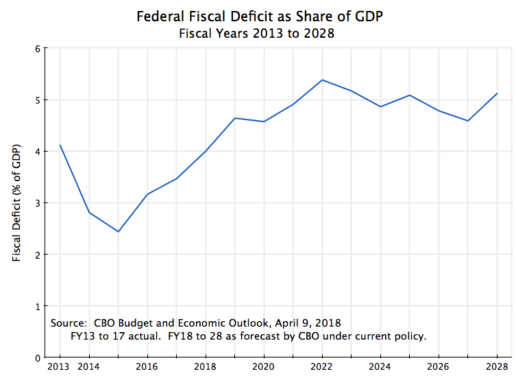
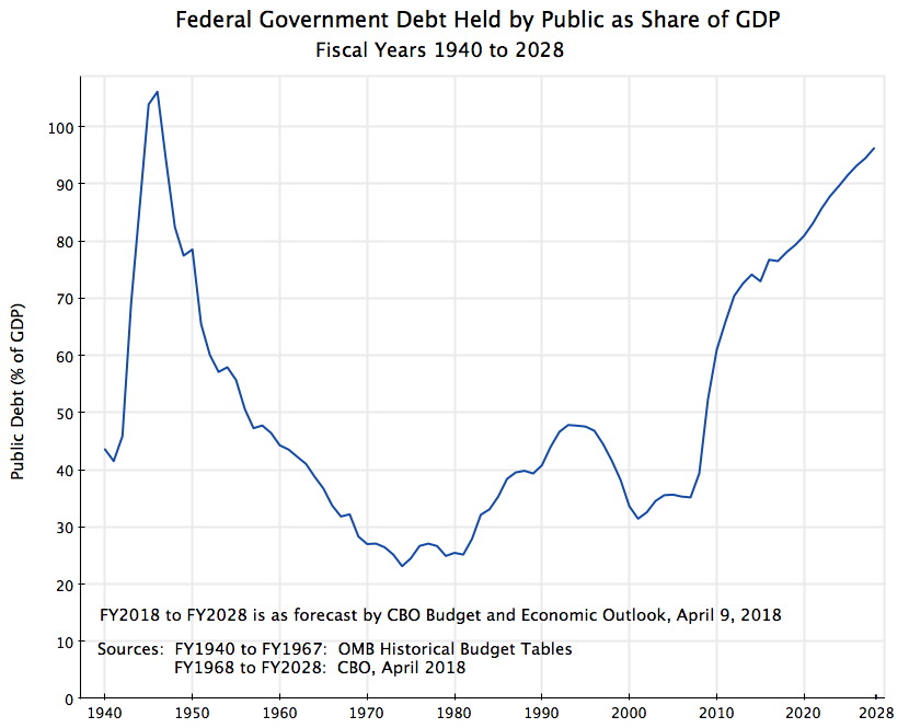
This leaves the budget deficit, and most agree that it really does need to be reduced in an economy that is now at full employment. Unfortunately, Trump and the Republican Congress have moved the budget in the exact opposite direction, primarily due to the huge tax cut passed last December, and to a lesser extent due to increases in certain spending (primarily for the military). As discussed in an earlier post on this blog, an increase in the budget deficit to a forecast 5% of GDP at a time when the economy is at full employment is unprecedented in peacetime.
What this implies for the trade balance is clear from the basic identity derived above. An increase in the budget deficit (a reduction in the budget balance) will lead, all else being equal, to an increase in the trade deficit (a reduction in the trade balance). And it might indeed be worse, as all else is not equal. The stated objective of slashing corporate taxes is to spur an increase in corporate investment. But if private investment were indeed to rise (there is in fact little evidence that it has moved beyond previous trends, at least so far), this would further worsen the trade balance (increase the trade deficit).
Would raising tariffs have an impact? One might argue that this would raise net Taxes paid, as tariffs on imports are a tax, which (if government spending is not then also changed) would reduce the budget deficit. While true, the extent of the impact would be trivially small. The federal government collected $35.6 billion in all customs duties and fees (tariffs and more) in FY2017 (see the OMB Historical Tables). This was less than 0.2% of FY2017 GDP. Even if all tariffs (and other fees on imports) were doubled, and the level of imports remained unchanged, this would only raise 0.2% of GDP. But the trade deficit was 2.9% of GDP in FY2017. It would not make much of a difference, even in such an extreme case. Furthermore, new tariffs are not being pushed by Trump on all imports, but only a limited share (and a very limited share so far). Finally, if Trump’s tariffs in fact lead to lower imports of the items being newly taxed, as he hopes, then tariffs collected can fall. In the extreme, if the imports of such items go to zero, then the tariffs collected will go to zero.
Thus, for several reasons, any impact on government revenues from the new Trump tariffs will be minor.
The notion that raising tariffs would be a way to eliminate the trade deficit is therefore confused. The trade balance will equal the difference between Domestic Savings and Domestic Investment. Adding in government, the trade balance will equal the difference between Domestic Private Savings and Domestic Private Investment, plus the equivalent for government (the Government Budget Balance, where a budget deficit will be a negative). Tariffs have little to no effect on these balances.
C. What Role Do Tariffs Play, Then?
Do tariffs then matter? They do, although not in the determination of the overall trade deficit. Rather, tariffs, which are a tax, will change the price of the particular import relative to the price of other products. If applied only to imports from some countries and not from others, one can expect to see a shift in imports towards those countries where the tariffs have not been imposed. And in the case when they are applied globally, on imports of the product from any country, one should expect that prices for similar products made in the US will then also rise. To the extent there are alternatives, purchases of the now more costly products (whether imported or produced domestically) will be reduced, while purchases of alternatives will increase. And there will be important distributional changes. Profits of firms producing the now higher priced products will increase, while the profits of firms using such products as an input will fall. And the real incomes of households buying any of these products will fall due to the higher prices.
Who wins and who loses can rapidly become turn into something very complicated. Take, for example, the new 25% tariff being imposed by the Trump administration on steel (and 10% on aluminum). The tariffs were announced on March 8, to take effect on March 23. Steel imports from Canada and Mexico were at first exempted, but later the Trump administration said those exemptions were only temporary. On March 22 they then expanded the list of countries with temporary exemptions to also the EU, Australia, South Korea, Brazil, and Argentina, but only to May 1. Then, on March 28, they said imports from South Korea would receive a permanent exemption, and Australia, Brazil, and Argentina were granted permanent exemptions on May 2. After a short extension, tariffs were then imposed on steel imports from Canada, Mexico, and the EU, on May 31. And while this is how it stands as I write this, no one knows what further changes might be announced tomorrow.
With this uneven application of the tariffs by country, one should expect to see shifts in the imports by country. What this achieves is not clear. But there are also further complications. There are hundreds if not thousands of different types of steel that are imported – both of different categories and of different grades within each category – and a company using steel in their production process in the US will need a specific type and grade of steel. Many of these are not even available from a US producer of steel. There is thus a system where US users of steel can apply for a waiver from the tariff. As of June 19, there have been more than 21,000 petitions for a waiver. But there were only 30 evaluators in the US Department of Commerce who will be deciding which petitions will be granted, and their training started only in the second week of June. They will be swamped, and one senior Commerce Department official quoted in the Washington Post noted that “It’s going to be so unbelievably random, and some companies are going to get screwed”. It would not be surprising to find political considerations (based on the interests of the Trump administration) playing a major role.
So far, we have only looked at the effects of one tariff (with steel as the example). But multiple tariffs on various goods will interact, with difficult to predict consequences. Take for example the tariff imposed on the imports of washing machines announced in late January, 2018, at a rate of 20% in the first year and at 50% should imports exceed 1.2 million units in the year. This afforded US producers of washing machines a certain degree of protection from competition, and they then raised their prices by 17% over the next three months (February to May).
But steel is a major input used to make washing machines, and steel prices have risen with the new 25% tariff. This will partially offset the gains the washing machine producers received from the tariff imposed on their product. Will the Trump administration now impose an even higher tariff on washing machines to offset this?
More generally, the degree to which any given producer will gain or lose from such multiple tariffs will depend on multiple factors – the tariff rates applied (both for what they produce and for what they use as inputs), the degree to which they can find substitutes for the inputs they need, and the degree to which those using the product (the output) will be able to substitute some alternative for the product, and more. Individual firms can end up ahead, or behind. Economists call the net effect the degree of “net effective protection” afforded the industry, and it can be difficult to figure out. Indeed, government officials who had thought they were providing positive protection to some industry often found out later that they were in fact doing the opposite.
Finally, imposing such tariffs on imports will lead to responses from the countries that had been providing the goods. Under the agreed rules of international trade, those countries can then impose commensurate tariffs of their own on products they had been importing from the US. This will harm industries that may otherwise have been totally innocent in whatever was behind the dispute.
An example of what can then happen has been the impact on Harley-Davidson, the American manufacturer of heavy motorcycles (affectionately referred to as “hogs”). Harley-Davidson is facing what has been described as a “triple whammy” from Trump’s trade decisions. First, they are facing higher steel (and aluminum) prices for their production in the US, due to the Trump steel and aluminum tariffs. Harley estimates this will add $20 million to their costs in their US plants. For a medium-sized company, this is significant. As of the end of 2017, Harley-Davidson had 5,200 employees in the US (see page 7 of this SEC filing). With $20 million, they could pay each of their workers $3,850 more. This is not a small amount. Instead, the funds will go to bolster the profits of steel and aluminum firms.
Second, the EU has responded to the Trump tariffs on their steel and aluminum by imposing tariffs of their own on US motorcycle imports. This would add $45 million in costs (or $2,200 per motorcycle) should Harley-Davidson continue to export motorcycles from the US to the EU. Quite rationally, Harley-Davidson responded that they will now need to shift what had been US production to one of their plants located abroad, to avoid both the higher costs resulting from the new steel and aluminum tariffs, and from the EU tariffs imposed in response.
And one can add thirdly and from earlier, that Trump pulled the US out of the already negotiated (but still to be signed) Trans-Pacific Partnership agreement. This agreement would have allowed Harley-Davidson to export their US built motorcycles to much of Asia duty-free. They will now instead be facing high tariffs to sell to those markets. As a result, Harley-Davidson has had to set up a new plant in Asia (in Thailand), shifting there what had been US jobs.
Trump reacted angrily to Harley-Davidson’s response to his trade policies. He threatened that “they will be taxed like never before!”. Yet what Harley-Davidson is doing should not have been a surprise, had any thought been given to what would happen once Trump started imposing tariffs on essential inputs needed in the manufacture of motorcycles (steel and aluminum), coming from our major trade partners (and often closest allies). And it is positively scary that a president should even think that he should use the powers of the state to threaten an individual private company in this way. Today it is Harley-Davidson. Who will it be tomorrow?
There are many other examples of the problems that have already been created by Trump’s new tariffs. To cite a few, and just briefly:
a) The National Association of Home Builders estimated that the 20% tariff imposed in 2017 on imports of softwood lumber from Canada added nearly $3,600 to the cost of building an average single-family home in the US and would, over the course of a year, reduce wages of US workers by $500 million and cost 8,200 full-time US jobs.
b) The largest nail manufacturer in the US said in late June that it has already had to lay off 12% of its workforce due to the new steel tariffs, and that unless it is granted a waiver, it would either have to relocate to Mexico or shut down by September.
c) As of early June, Reuters estimated that at least $2.5 billion worth of investments in new utility-scale solar installation projects had been canceled or frozen due to the tariffs Trump imposed on the import of solar panel assemblies. This is far greater than new investments planned for the assembly of such panels in the US. Furthermore, the jobs involved in such assembly work are generally low-skill and repetitive, and can be automated should wages rise.
So there are consequences from such tariffs. They might be unintended, and possibly not foreseen, but they are real.
But would the imposition of tariffs necessarily reduce the trade deficit, as Trump evidently believes? No. As noted above, the trade deficit would only fall if the tariffs would, for some reason, increase domestic savings or reduce domestic investment. But tariffs do not enter directly into those factors. Indirectly, one could map out some chains of possible causation, but these changes in some set of tariffs (even if broadly applied to a wide range of imports) would not have a major effect on overall domestic savings or investment. They could indeed even act in the opposite direction.
Households, to start, will face higher prices from the new tariffs. To try to maintain their previous standard of living (in real terms) they would then need to spend more on what they consume and hence would save less. This, by itself, would reduce domestic savings and hence would increase the trade deficit to the extent there was any impact.
The impacts on firms are more various, and depend on whether the firm will be a net winner or loser from the government actions and how they might then respond. If a net winner, they have been able to raise their prices and hence increase their profits. If they then save the extra profits (retained earnings), domestic savings would rise and the trade deficit would fall. But if they increase their investments in what has now become a more profitable activity (and that is indeed the stated intention behind imposing the tariffs), that response would lead to an increase in the trade deficit. The net effect will depend on whether their savings or their investment increases by more, and one does not know what that net change might be. Different firms will likely respond differently.
One also has to examine the responses of the firms who will be the net losers from the newly imposed tariffs. They will be paying more on their inputs and will see a reduction in their profits. They will then save less and will likely invest less. Again, the net impact on the trade deficit is not clear.
The overall impact on the trade deficit from these indirect effects is therefore uncertain, as one has effects that will act in opposing directions. In part for this reason, but also because the tariffs will affect only certain industries and with responses that are likely to be limited (as a tariff increase today can be just as easily reversed tomorrow), the overall impact on the trade balance from such indirect effects are likely to be minor.
Increases in individual tariffs, such as those being imposed now by Trump, will not then have a significant impact on the overall trade balance. But tariffs still do matter. They change the mix of what is produced, from where items will be imported, and from where items will be produced for export (as the Harley-Davidson case shows). They will create individual winners and losers, and hence it is not surprising to see the political lobbying as has grown in Washington under Trump. Far from “draining the swamp”, Trump’s trade policy has made it critical for firms to step up their lobbying activities.
But such tariffs do not determine what the overall trade balance will be.
D. What Role Does Foreign Investment Play in the Determination of the Trade Balance?
While tariffs will not have a significant effect on the overall trade balance, foreign investment (into the US) will. To see this, we need to return to the basic macro balance derived in Section B above, but generalize it a bit to include all foreign financial flows.
The trade balance is the balance between exports and imports. It is useful to generalize this to take into account two other sources of current flows in the national income and product accounts which add to (or reduce) the net demand for foreign exchange. Specifically, there will be foreign exchange earned by US nationals working abroad plus that earned by US nationals on investments they have made abroad. Economists call this “factor services income”, or simply factor income, as labor and capital are referred to as factors of production. This is then netted against such income earned in the US by foreign nationals either working here or on their investments here. Second, there will be unrequited transfers of funds, such as by households to their relatives abroad, or by charities, or under government aid programs. Again, this will be netted against the similar transfers to the US.
Adding the net flows from these to the trade balance will yield what economists call the “current account balance”. It is a measure of the net demand for dollars (if positive) or for foreign exchange (if a deficit) from current flows. To put some numbers on this, the US had a foreign trade deficit of $571.6 billion in 2017. This was the balance between the exports and imports of goods and services (what economists call non-factor services to be more precise, now that we are distinguishing factor services from non-factor services). It was negative – a deficit. But the US also had a surplus in 2017 from net factor services income flows of $216.8 billion, and a deficit of $130.2 billion on net transfers (mostly from households sending funds abroad). The balance on current account is the sum of these (with deficits as negatives and surpluses as positives) and came to a deficit of $485.0 billion in 2017, or 2.5% of GDP. As a share of GDP, this deficit is significant but not huge. The UK had a current account deficit of 4.1% of GDP in 2017 for example, while Canada had a deficit of 3.0%.
The current account for foreign transactions, basically a generalization of the trade balance, is significant as it will be the mirror image of the capital account for foreign transactions. That is, when the US had a current account deficit of $485.0 billion (as in 2017), there had to be a capital account surplus of $485.0 billion to match this, as the overall purchases and sales of dollars in foreign exchange transactions will have to balance out, i.e. sum to zero. The capital account incorporates all transactions for the purchase or sale of capital assets (investments) by foreign entities into the US, net of the similar purchase or sale of capital assets by US entities abroad. When the capital account is a net positive (as has been the case for the US in recent decades), there is more such investment going into the US than is going out. The investments can be into any capital assets, including equity shares in companies, or real estate, or US Treasury or other bonds, and so on.
But while the two (the current account and the capital account) have to balance out, there is an open question of what drives what. Look at this from the perspective of a foreigner, wishing to invest in some US asset. They need to get the dollars for this from somewhere. While this would be done by means of the foreign exchange markets, which are extremely active (with trillions of dollars worth of currencies being exchanged daily), a capital account surplus of $485 billion (as in 2017) means that foreign entities had to obtain, over the course of the year, a net of $485 billion in dollars for their investments into the US. The only way this could be done is by the US importing that much more than it exported over the course of the year. That is, the US would need to run a current account deficit of that amount for the US to have received such investment.
If there is an imbalance between the two (the current account and the capital account), one should expect that the excess supply or demand for dollars will lead to changes in a number of prices, most directly foreign exchange rates, but also interest rates and other asset prices. These will be complex and we will not go into here all the interactions one might then have. Rather, the point to note is that a current account deficit, even if seemingly large, is not a sign of disequilibrium when there is a desire on the part of foreign investors to invest a similar amount in US markets. And US markets have traditionally been a good place to invest. The US is a large economy, with markets for assets that are deep and active, and these markets have normally been (with a few exceptions) relatively well regulated.
Foreign nationals and firms thus have good reason to invest a share of their assets in the US markets. And the US has welcomed this, as all countries do. But the only way they can obtain the dollars to make these investments is for the US to run a current account deficit. Thus a current account deficit should not necessarily be taken as a sign of weakness, as Trump evidently does. Depending on what governments are doing in their market interventions, a current account deficit might rather be a sign of foreign entities being eager to invest in the country. And that is a good sign, not a bad one.
E. An “Exorbitant Privilege”
The dollar (and hence the US) has a further, and important, advantage. It is the world’s dominant currency, with most trade contracts (between all countries, not simply between some country and the US) denominated in dollars, as are contracts for most internationally traded commodities (such as oil). And as noted above, investments in the US are particularly advantageous due to the depth and liquidity of our asset markets. For these reasons, foreign countries hold most of their international reserves in dollar assets. And most of these are held in what have been safe, but low yielding, short-term US Treasury bills.
As noted in Section D above, those seeking to make investments in dollar assets can obtain the dollars required only if the US runs a current account deficit. This is as true for assets held in dollars as part of a country’s international reserves as for any other investments in US dollar assets. Valéry Giscard d’Estaing in the 1960s, then the Minister of Finance of France, described this as an “exorbitant privilege” for the US (although this is often mistakenly attributed Charles de Gaulle, then his boss as president of France).
And it certainly is a privilege. With the role of the dollar as the preferred reserve currency for countries around the world, the US is able to run current account deficits indefinitely, obtaining real goods and services from those countries while providing pieces of paper generating only a low yield in return. Indeed, in recent years the rate of return on short-term US Treasury bills has generally been negative in real terms (i.e. after inflation). The foreign governments buying these US Treasury bills are helping to cover part of our budget deficits, and are receiving little to nothing in return.
So is the US a “piggybank that everybody is robbing”, as Trump asserted to necessarily be the case when the US is has a current account deficit? Not at all. Indeed, it is the precise opposite. The current account deficit is the mirror image of the foreign investment inflows coming into the US. To obtain the dollars needed to do this those countries must export more real goods to the US than they import from the US. The US gains real resources (the net exports), while the foreign entities then invest in US markets. And for governments obtaining dollars to hold as their international reserves, those investments are primarily in the highly liquid and safe, short-term US Treasury bills, despite those assets earning low or even negative returns. This truly is an “exorbitant privilege”, not a piggybank being robbed.
Indeed, the real concern is that with the mismanagement of our budget (tax cuts increasing deficits at a time when deficits should be reduced) plus the return to an ideologically driven belief in deregulating banks and other financial markets (such as what led to the financial and then economic collapse of 2008), the dollar may lose its position as the place to hold international reserves. The British pound had this position in the 1800s and then lost it to the dollar due to the financial stresses of World War I. The dollar has had the lead position since. But others would like it, most openly by China and more quietly Europeans hoping for such a role for the euro. They would very much like to enjoy this “exorbitant privilege”, along with the current account deficits that privilege conveys.
F. Summary and Conclusion
Trump’s beliefs on the foreign trade deficit, on the impact of hiking tariffs, and on who will “win” in a trade war, are terribly confused. While one should not necessarily expect a president to understand basic economics, one should expect that a president would appoint and listen to advisors who do. But Trump has not.
To sum up some of the key points:
a) The foreign trade balance will always equal the difference between domestic savings and domestic investment. Or with government accounts split out, the trade balance will equal the difference between domestic private savings and domestic private investment, plus the government budget balance. The foreign trade balance will only move up or down when there is a change in the balance between domestic savings and domestic investment.
b) One way to change that balance would be for the government budget balance to increase (i.e. for the government deficit to be reduced). Yet Trump and the Republican Congress have done the precise opposite. The massive tax cuts of last December, plus (to a lesser extent) the increase in government spending now budgeted (primarily for the military), will increase the budget deficit to record levels for an economy in peacetime at full employment. This will lead to a bigger trade deficit, not a smaller one.
c) One could also reduce the trade deficit by making the US a terrible place to invest in. This would reduce foreign investment into the US, and hence the current account deficit. In terms of the basic savings/investment balance, it would reduce domestic investment (whether driven by foreign investors or domestic ones). If domestic savings was not then also reduced (a big if, and dependant on what was done to make the US a terrible place to invest in), this would lead to a similar reduction in the trade deficit. This is of course not to be taken seriously, but rather illustrates that there are tradeoffs. One should not simplistically assume that a lower trade deficit achieved by any means possible is good.
d) It is also not at all clear that one should be overly concerned about the size of the trade and current account deficits, at where they are today. The US had a trade deficit of 2.9% of GDP in 2017 and a current account deficit of 2.5% of GDP. While significant, these are not huge. Should they become much larger (due, for example, to the forecast increases in government budget deficits to record levels), they might rise to problematic levels. But at the current levels for the current account deficit, we have seen the markets for foreign exchange and for interest rates functioning pretty well and without overt signs of concern. The dollars being made available through the current account deficit have been bought up and used for investments in US markets.
e) Part of the demand for dollars to be invested and held in the US markets comes from the need for international reserves by governments around the world. The dollar is the dominant currency in the world, and with the depth and liquidity of the US markets (in particular for short-term US Treasury bills) most of these international reserves are held in dollars. This has given the US what has been called an “exorbitant privilege”, and permits the US to run substantial current account deficits while providing in return what are in essence paper assets yielding just low (or even negative) returns.
f) The real concern should not be with the consequences of the dollar playing such a role in the system of international trade, but rather with whether the dollar will lose this privileged status. Other countries have certainly sought this, most openly by China but also more quietly for the euro, but so far the dollar has remained dominant. But there are increasing concerns that with the mismanagement of the government budget (the recent tax cuts) plus ideologically driven deregulation of banks and the financial markets (as led to the 2008 financial collapse), countries will decide to shift their international reserves out of the dollar towards some alternative.
g) What will not reduce the overall trade deficit, however, is selective increases in tariff rates, as Trump has started to do. Such tariff increases will shift around the mix of countries from where the imports will come, and/or the mix of products being imported, but can only reduce the overall trade deficit to the extent such tariffs would lead somehow to either higher domestic savings and/or lower domestic investment. Tariffs will not have a direct effect on such balances, and indirect effects are going to be small and indeed possibly in the wrong direction (if the aim is to reduce the deficits).
h) What such tariff policies will do, however, is create a mess. And they already have, as the Harley-Davidson case illustrates. Tariffs increase costs for US producers, and they will respond as best they can. While the higher costs will possibly benefit certain companies, they will harm those using the products unless some government bureaucrat grants them a special exemption.
But what this does lead to is officials in government picking winners and losers. That is a concern. And it is positively scary to have a president lashing out and threatening individual firms, such as Harley-Davidson, when the firms respond to the mess created as one should have expected.

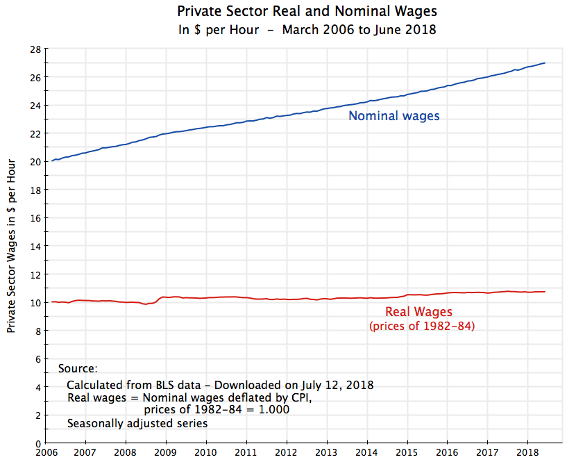
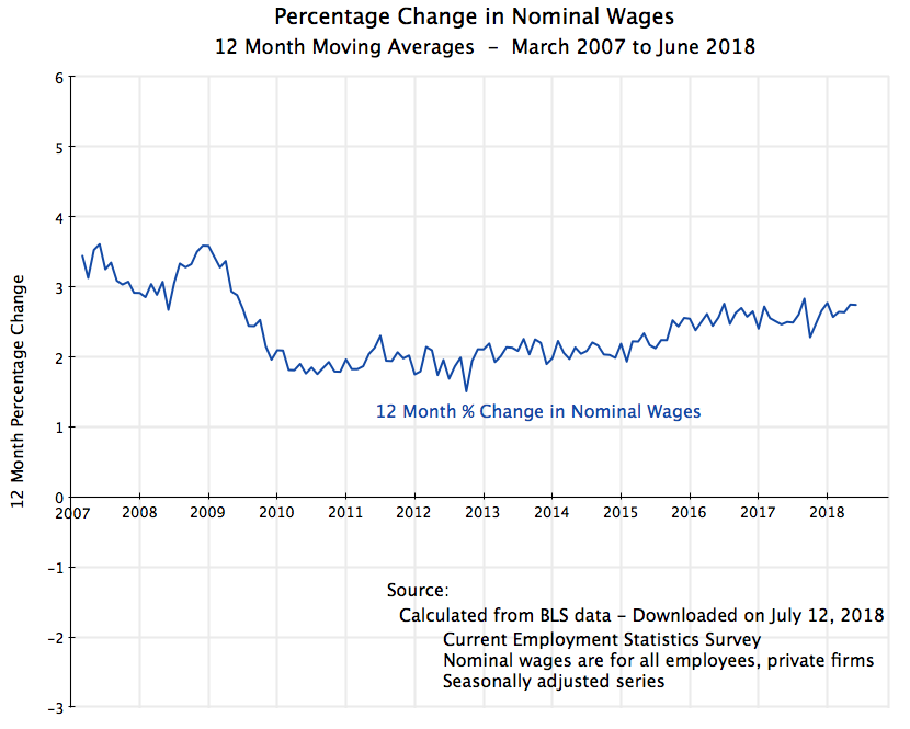 Note that the date labels are for the end of each period. Thus the point labeled at the start of 2008 will cover the percentage change in the nominal wage between January 2007 and January 2008. And the starting date label for the chart will be March 2007, which covers the period from March 2006 (when the data series begins) to March 2007.
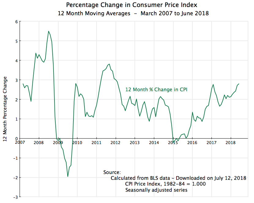 But note that “larger” should be interpreted in a relative sense. The absolute changes were generally not all that large (with some exceptions), and can mostly be attributed to changes in the prices of a limited number of volatile commodities, namely for food items and energy (oil). The prices of such commodities go up and down, but over time they even out. Thus for understanding inflationary trends, analysts will often focus instead on the so-called “core CPI”, which excludes food and energy prices. For the full period being examined here, the regular CPI rose at a 1.88% annual pace while the core CPI rose at a 1.90% pace. Within round-off, these are essentially the same.
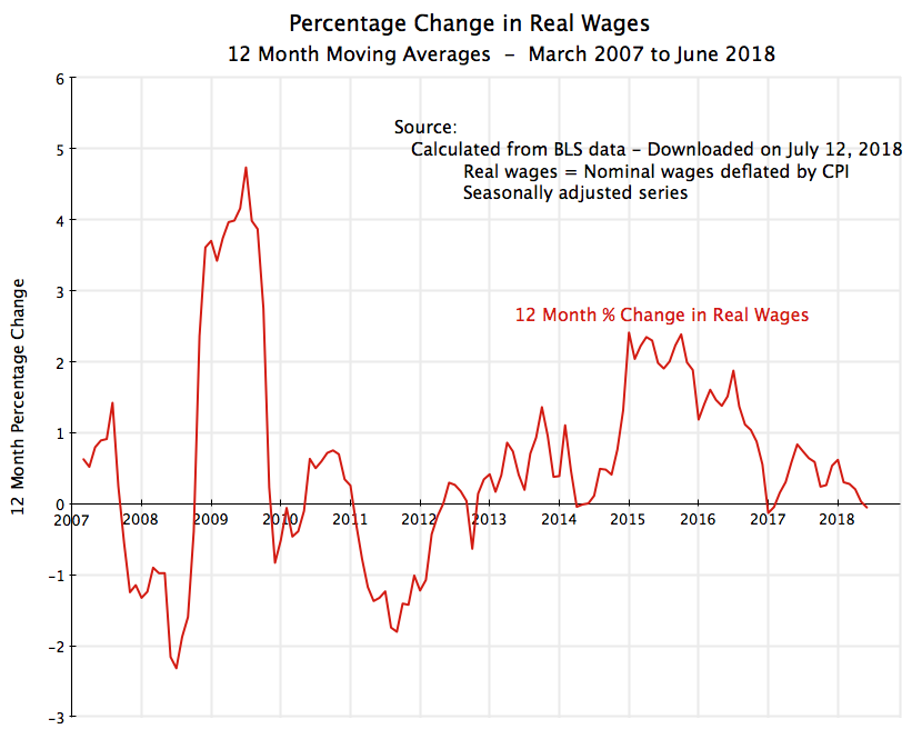 With the relatively steady changes in average nominal wages, year to year, the fluctuations will basically be the mirror image of what has been happening to inflation. When prices fell, real wages rose, and when prices rose more than normal, real wages fell.


You must be logged in to post a comment.