The Growing Inequality in Wealth in the US, Part 1 – Basic Facts

Chart 1

A.  Introduction

The extreme, and growing, inequality in wealth ownership in the US has been receiving increasing attention.  In its most recent annual listing of the 400 most wealthy Americans (from September 15, 2026), Forbes estimates that 15 individuals (and their immediate families) each have a wealth of $100 billion or more, seven have a wealth of $200 billion or more, and the top one – Elon Musk – had a wealth (as of the date of publication) of over $900 billion.  Concern with such concentration of wealth has also grown as a number of these ultra-wealthy individuals have become increasingly politically active, using their wealth in ways that can determine election outcomes and overwhelm basic democratic institutions.  This became especially evident in the 2024 presidential election, with consequences that are now clear.

This post, and several to follow, will review the basic data that estimate the inequality in wealth holdings and how that inequality has grown in recent decades.  This first post will look at wealth per household (more precisely net worth, but the terms will be used interchangeably) with the households ranked by their level of wealth from least to most:  the bottom 50%, the 50 to 90%, the 90 to 99%, the 99.0 to 99.9%, and the top 0.1%.

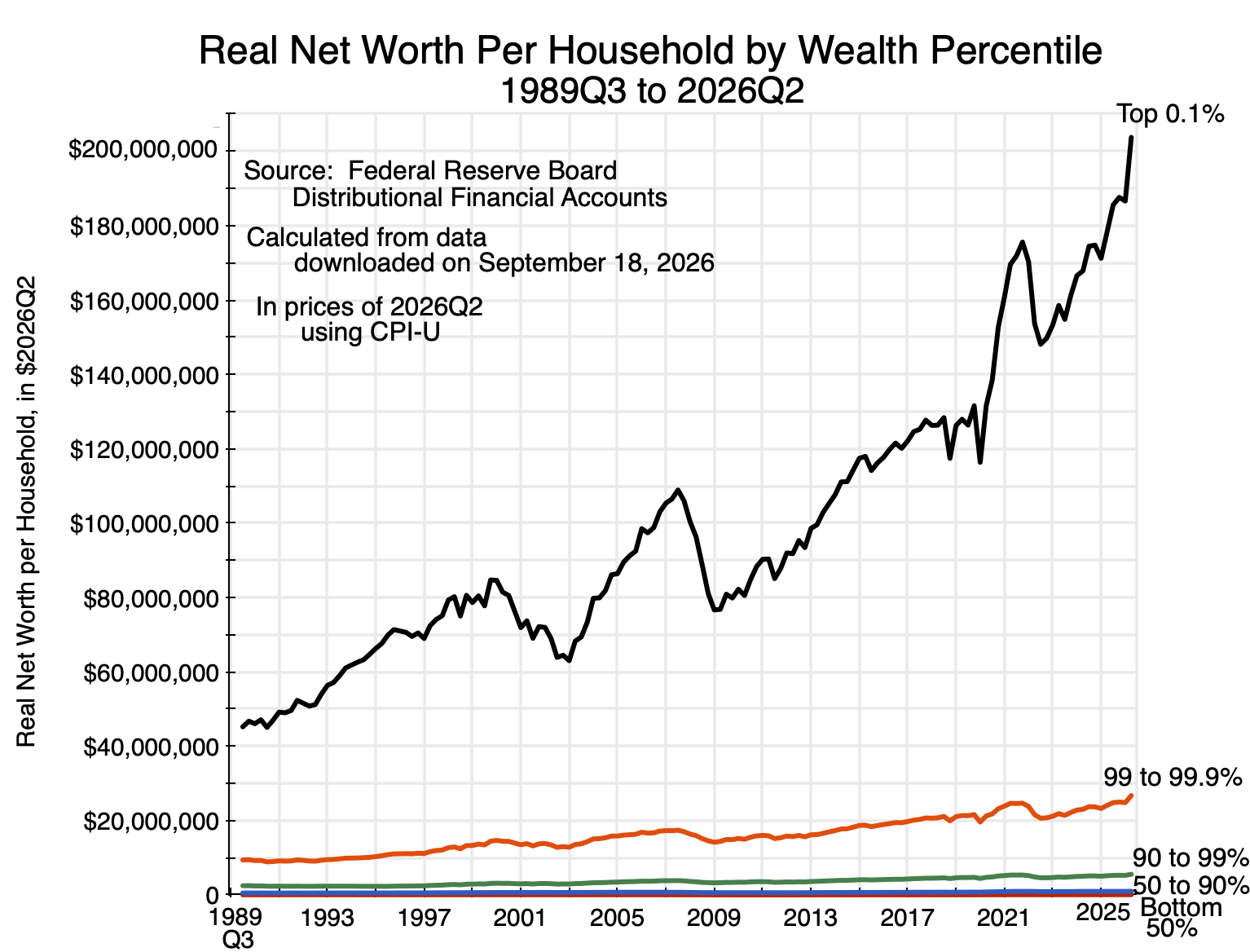
The chart at the top of this post shows how that net worth has grown (in real terms) over the last several decades.  Because of the immense wealth of the top 0.1% – whose average net worth grew to over $200 million per household – it is hard to see on the chart the average wealth of the bottom 99% of the population.  Their net worth is just too small.  Charts below will split out the bottom 99% to show their histories, but the point is that the disparity between the top 0.1% and the rest is so large that – other than for the top 1% – their average holdings disappear on the scale of the chart.

The post will first discuss in Section B below the data for these estimates.  They were calculated from data estimated by staff at the Federal Reserve Board and released as its Distributional Financial Accounts.  This source is widely considered the best set of estimates on household wealth available for the US.  These are, of course, estimates, however, and while the best available, it is important still to recognize their limitations.  Wealth is difficult to estimate, for both conceptual and practical reasons.

Section C will then present the basic estimates of per-household wealth (net worth) when grouped by households ranked by the wealth they hold.  The figures going back to 1989Q3 for all five groups the Fed distinguishes are as in the chart at the top of this post, and charts will then be provided also for the bottom 99% (and its sub-groups) and for the bottom 50%.  Each has a story to tell.

Section D examines how the wealth estimates have changed over time in real terms and per household relative to what they were in the earliest period in this data series (1989Q3).  Inequality was already high in 1989, but then grew much more.  Section E will decompose the figures for average overall wealth, linking their increase to the growth in GDP over the period, to the increasing share of profits in GDP (at the expense of wages), and to the increase in how that wealth is valued as a multiple of the profits the owners of the assets are entitled to.

Section F will conclude.  Future posts will examine other aspects of wealth holdings, using the same Fed data, including on wealth holdings when households are ranked by their income levels rather than their wealth levels, and on wealth holdings at the same age for different generations – i.e. for Baby Boomers compared to generations before and after.  A final post will then examine what might – or might not – be done through policy to address these issues.

B.  The Fed’s Distributional Financial Accounts

The measurement of wealth is not at all straightforward, and poses both conceptual and practical issues.  This is in contrast to the measurement of incomes.  For incomes, there are actual market transactions where firms earn revenues from what they sell.  Out of those revenues the firms pay a portion for the inputs used and for the wages of their employees, with the remainder then being the gross profits that will cover taxes, the interest they pay on their debt, and their investment costs (counted as depreciation).  What remains is their net profits.  All of these transactions (other than depreciation) are measurable in cash being transferred and can be observed.

The measurement of wealth is different.  Wealth is the value that others would be willing to pay for the assets owned.  That is not observed and can only be estimated.  Guessed may be a better term.  It is also in a fundamental sense socially determined, as the measured value of the wealth is not inherent in the asset itself, but rather an estimate of what others – given the state of the economy, their expectations of what the future might be, the availability of financing, and other such factors – might be willing to pay for the asset.  The transfer of the asset does not take place, however, and hence cannot be observed in the manner that incomes are observed.  The value can only be estimated as a hypothetical.

Thus if someone is willing to pay twice as much for an asset (perhaps real estate, or a company, or whatever) than what it was valued at the previous day, the owner of the asset would be richer.  His wealth would be greater.  But nothing fundamental has changed in the economy; the assets are all the same as before.  Only the valuation has changed.

In the face of such issues, statisticians do the best they can.  They need to make assumptions about what others might be willing to pay for the assets.  And they can assemble data on transfers of assets that have recently taken place and hence can be observed, where those assets may be similar – to a greater or lesser degree – to those they are trying to value.  This can inform – to some extent – the valuations they assign to assets that did not change hands.

The calculations discussed in this post (and those that follow in this series) are based on data assembled by staff at the Board of Governors of the Federal Reserve System in Washington, DC, and specifically its Distributional Financial Accounts (DFA).  The DFA estimates are published quarterly, usually about 11 weeks after the end of each calendar quarter.  The accounts for the second quarter of 2026 were released on September 18, and provide estimates for wealth held by households as of the end of the quarter, i.e. on June 30.

The DFA data sets include quarterly data going back to the third quarter of 1989, but were only first produced starting in 2019.  They are based on a combination of two other data sets produced by staff at the Fed Board of Governors, the Survey of Consumer Finances (SCF) – a survey undertaken once every three years –  and the quarterly Financial Accounts of the United States (FA).

The SCF is a survey of households undertaken on behalf of the Fed where household assets and liabilities are recorded in detail, along with household income and characteristics of the household such as the age, education, race, and similar of its members.  Because of this, the Fed can then produce estimates of wealth not simply of households in general, but also of households categorized by their income, their age, education, and/or race, and similar.

A representative sample of households across the country is chosen for the SCF, along with an oversampling of higher-income households in order to get meaningful sample sizes of the more wealthy households that hold a substantial share of household wealth.

The response rate of the general sample is reasonably good – at about 70% – but that for the oversampled wealthy households is only 10%.  This may lead to biases in the results.  While it would not matter if the wealthy households not responding were random (one could then simply start with a sample size ten times larger), it is likely that the relatively more wealthy households within that group are less likely to respond.  The share of the nation’s wealth held by the most wealthy would then be underestimated.  Despite this possible bias in the estimates, we will see below that the share held by the most wealthy groups is nonetheless extremely high.

A point to note is that the SCF specifically excludes any sampling of the extremely wealthy households on the Forbes 400 list of richest Americans.  This might be due to privacy concerns, or simply the recognition that they would be unlikely to respond to the SCF survey even if asked.  However, the DFA accounts specifically add them back in, with assets and liabilities either obtained from Forbes or drawn from the same sources used by Forbes.  The net worth of the top 400 is significant.  In the most recent September 2026 ranking, their total net worth came to $8 trillion.  The DFA estimate of the net worth of the top 0.1% of households as of June 30, 2026, was $28 trillion.  Thus the top 400 alone account for 29% of the total wealth of the group, even though they account for less than 0.3% of the approximately 135,000 households in the top 0.1%.

The SCF is, as noted, conducted only once every three years.  To arrive at the quarterly estimates, the Fed staff use the quarterly Financial Accounts of the United States (FA) data to estimate how the wealth holdings of the households in the groupings analyzed may have changed quarter to quarter.  The FA accounts date back to 1955, and were formerly called the Flow of Funds Accounts.  They track – for the nation as a whole – both the stocks and flows of capital assets (both real and financial) in all their forms across economic sectors such as households, businesses, governments, and financial intermediaries.  They are normally released ten weeks after the end of the quarter, and present financial flows during that quarter along with end-of-period stocks.

The DFA estimates combine the triennial SCF estimates on wealth holdings of categories of households with the quarterly FA estimates of total assets and liabilities held by households in the country as a whole.  But this is not always a simple scaling, for several reasons.  For a full discussion, see this chapter from a NBER conference held in March 2020 (and published in 2022) where Fed staff describe in some detail how the then new DFA accounts were assembled.

Arriving at household holdings of wealth – both assets and liabilities – consistent with national-level estimates of the totals of such assets and liabilities in the economy is not always straightforward.  A couple of examples illustrate this.

One is the accounting of the assets backing up commitments to retirees in defined benefit pension plans.  The SCF does not attempt to include at the household level the assets held in such schemes.  Workers expect they will receive a pension of some amount, which will be tied to how many years they ended up working for the firm and what their final income was (often averaged over some period, such as their final three years).  They will have little idea what assets are being invested to back up those commitments.  But at the national level, the assets of the company pension plans backing up those commitments have been invested and are reflected in the totals in the FA accounts.

To resolve this, the DFA makes an estimate of what a household’s share of the assets held by the pension fund managers would be given the characteristics of the households.  For those who are already retired and are receiving such a pension, plus for those who expect to receive a pension at a certain level based on their past employment with some firm, they calculate the present discounted value (which will depend on their age) of their expected future pension benefits.  They then subtract those present value totals from the assets of the defined benefit pension plans at the national level to arrive at a figure for the pensions of workers still employed, who will start to receive pension benefits once they retire at some future date. They use a similar approach for the determination of the value at the household level of wealth held indirectly in annuity schemes and in life and other insurance plans.  This approach can be easily criticized, but is probably the best that can be done.

As another example of the type of assumptions they had to make, there is an issue with how equity in privately held businesses as well as closely-held corporate entities should be valued.  The SCF reported figures based on the household responses for both the cost basis of such equity and for what the households believed the market value would be.  Aggregated to the national level, the market value estimates were well above the totals in the FA accounts while the cost basis estimates were well below.  However, the average of the two turned out to be close, so they used that.

It should be noted that while estimates are made of the value to the household of the assets held (directly or indirectly) in their defined benefit pension plans as well as their defined contribution plans (401k’s, IRAs, and so on) and annuities from insurers, the DFA accounts do not include the implicit value of their Social Security retirement (and other) benefits.  But the value of those Social Security commitments are significant, and especially so (as a share of their total wealth) for lower-income households.

To illustrate, a standard rule-of-thumb in retirement calculations is to spend each year no more than 4% of the balance of assets held in the retirement accounts at the time of retirement.  The remaining assets will continue to grow in value, but at that 4%, retirees are unlikely to outlive the savings they had to cover retirement.  Based on this, one can calculate the assets that would be required in a private pension savings account to cover benefits equal to those paid by Social Security.

As of December, 2025, the average monthly benefits paid to retirees, along with the average paid to the bottom 50% of retirees and top 50%, were:

Average Monthly Benefit

Annual Equivalent

Capital-Value Using 4% Rule

All Retired Workers

$2,071

$24,854

$621,350

Bottom 50%

$1,338

$16,060

$401,505

Top 50%

$2,813

$33,761

$844,017

Source:  Calculated from data at Social Security – Beneficiaries by benefit level.  For December 2025.

To cover the average benefit to retirees of $2,071 per month, assets of over $620,000 would have been needed if one followed the 4% rule.  For the bottom 50% of retirees (bottom 50% of the recipients of Social Security benefits), it would have been over $400,000, and over $840,000 for the top 50%.  These could be counted as part of household wealth (assuming Social Security keeps to its commitments – which certainly can be done but will require Congress to act).

These are significant amounts.  As will be discussed in the following section below, the average net worth as of June 30, 2026, of the bottom 50% of households (as ranked by their net worth) is only $63,000 in the DFA figures.  For those in the 50 to 90% percentile, the average net worth was $988,000.

At the same time, keep in mind that the assets required by the 4% rule to match what Social Security is paying retirees would be the assets as of the year they retire and start collecting Social Security retirement benefits.  Any individual builds up this entitlement to benefits over their working life, and thus the equivalent value when they are younger would be proportionally less.  Similarly, retirement assets will be drawn down during the years one is retired, so the equivalent assets as one ages after retirement will then also be less.

However, the important point is that Social Security could be seen as a significant addition to household wealth, and especially so for the least wealthy.  The DFA could have included that implicit wealth (with then a suitable adjustment in the treatment of the Social Security Trust Account in the federal government accounts) just as they did for private defined contribution pension plans, but chose not to.

I have given these examples to make clear that the wealth figures really are estimates, where those estimates need to be based on assumptions that can be questioned.  The approach taken is probably the best that has been done to estimate the distribution of wealth in the US, but the limitations should not be forgotten.

C.  Real Net Worth per Household, Stratified by Rank in Terms of Net Worth

There is extreme disparity in the distribution of wealth in the US.  Specific figures by category of household may provide a better sense of this, along with the ownership of the types of assets of each group.  As of the end of the second quarter of 2026:

2026Q2 per Household – in $thousands

Bottom 50%

50 to 90%

90 to 99%

99.0 to 99.9%

Top 0.1%

A.  Total Assets

$152

$1,153

$5,906

$27,454

$205,938

1) Real Estate

$71

$429

$1,240

$3,876

$14,377

2) Consumer durables

$32

$71

$158

$347

$5,413

3) Bank deposits & Money mkt accts

$12

$113

$583

$2,345

$17,790

4) Bonds/Loans

$1

$24

$214

$1,066

$9,418

5) Equities

$8

$180

$2,412

$17,164

$153,056

6) Retirement accts

$19

$304

$1,210

$2,234

$3,873

7) Other

$8

$30

$90

$421

$2,012

B. Total Liabilities

$89

$164

$346

$732

$2,200

1) Home mortgages

$47

$126

$280

$373

$857

2) Consumer credit

$39

$33

$43

$92

$383

3) Other

$3

$5

$23

$267

$960

C.  Net Worth

$63

$988

$5,559

$26,722

$203,738

o/w Net Real Estate

$25

$303

$959

$3,503

$13,520

Source:  Calculated from the data at Fed Board of Governors, Distributional Financial Accounts.  Downloaded September 18, 2026.

Households are ranked here by their net worth – from those with the least (and indeed negative) net worth to those with the most.  The DFA shows the totals held in categories for the bottom 50% of households, for those ranked between 50 and 90%, between 90 and 99%, between 99.0 and 99.9%, and for the top 0.1%, along with the number of households in each group (so one can calculate the per household averages).  As of the end of 2026Q2, there were approximately 135 million households in the US, so the bottom 50% covered the 67.5 million with the least net worth, and then so on to the top 0.1% with approximately 135,000 households.

The DFA data (in what is made publicly available) identify 15 categories of assets and 5 categories of liabilities.  The table above aggregates some of these into broader categories of interest.  The figures shown here are rounded to thousands, and for the reasons discussed in the preceding section of this post, need to be taken as approximate estimates.

Keep in mind also that these are averages over the households in each of the given categories.  The minimum net worth to be included in the categories (in 2022Q2 – the date of the most recent SCF survey used for this categorization) was $240,000 for the 50 to 99% group, $2.1 million for the 90 to 99% group, $11.0 million for the 99.0 to 99.9% group, and $46 million for the top 0.1%.

Also keep in mind that the categories cover individuals of all ages.  The trends over time do not follow the experience of any given individual, who might start out their working life with a very low net worth – and thus is in the bottom 50% of households – but who then accumulates wealth as they grow older and ends up in one of the wealthier groups.  Rather, the figures on the wealth holdings over time are for those in each of the groups (the bottom 50%, the 50 to 90%, and so on) at each point in time.

Furthermore, because the distribution of net worth is highly skewed to the right – both overall and within each category of net worth – the average holdings of a group will be greater than the median holdings.  That is, the median holding – the net worth where half of the households in the group hold less and half hold more – will be less than the averages shown in this table.  Since the DFA files released by the Fed only show total holdings (in nominal terms) and the number of households in each group, one can calculate averages but not medians.

The one exception where a median can be found is the dividing line in net worth between the bottom 50% of households and the next group up (the 50 to 90%).  As noted above, that dividing line in 2022Q2 was $240,000.  Since 50% of households have a net worth less than this, that will be the median for the nation as a whole.  But the average net worth of households in the nation as a whole was $1,043,000 as of the end of 2022Q2.  The average is more than four times the median.  As of the end of 2026Q2, the average net worth was $1,373,000.  (The figures in this paragraph are all in current price terms.)

But even with the qualifiers on the impact of age and the difference between the average and the median due to the skewness of the distributions, I still find it mind-boggling that the DFA estimates indicate that the top 0.1% – 135,000 households in the US – have on average a net worth as of the end of June 2026 of $203.7 million.

The chart at the top of this post shows how the average net worth of households ranked by their wealth percentile has grown since 1989Q3.  To allow for meaningful comparisons over time, these have been adjusted for inflation using the CPI-U index – the most commonly used consumer price index measure in the US.  They are expressed in terms of the prices of 2026Q2.

The average net worth of the top 0.1% of wealth-holders rose from $45.2 million in 1989Q3 (in prices of 2026Q2) to $203.7 million as of the end of 2026Q2.  The substantial increase in wealth of those in the 99.0 to 99.9% group can also be seen in the chart (from $9.4 million on average at the start to $26.7 million now).  But the scale of the chart is such that what happened for those in the bottom 99% is not clear.

Limiting the chart to just the groups in the bottom 99%, one has:
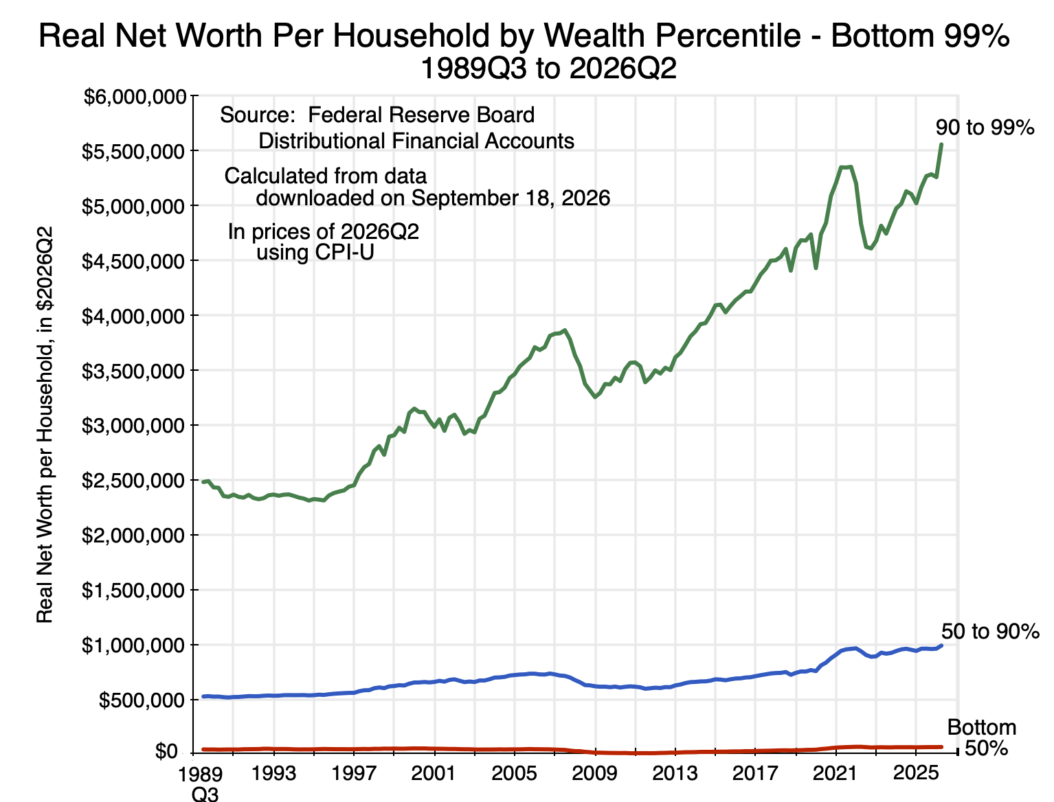
Chart 2

The average net worth of the 90 to 99% group rose over the period from $2.5 million to $5.6 million as of the end of 2026Q2.  The average net worth for the 50 to 90% group rose from $524,000 to $988,000.

The line for the bottom 50% is still not clear, so in a chart on its own:
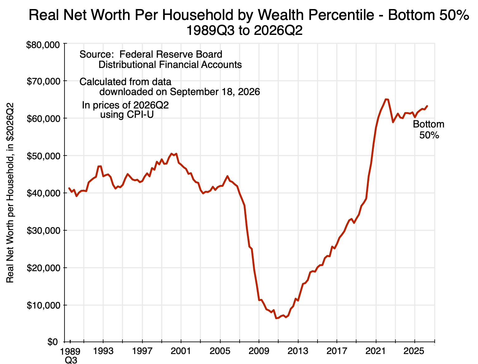
Chart 3

The path is far from steady:  While average net worth for the bottom 50% rose over the full period from $41,200 to $63,300, it fell to a low of just $6,400 in 2010Q4 as a result of the 2008/09 economic and financial crisis.  This primarily reflected the crash in real estate values – assets which account for a disproportionate share of the wealth of the bottom 50%.  The average net value of their real estate wealth (i.e. the value of their real estate assets less that owed on home mortgages) was a negative $15,850 at the end of 2010.

Furthermore, while their net worth then recovered, it did not recover fully until 2020.  The average net worth of the bottom 50% was $44,500 in 2005Q4, and an even higher $50,500 in 2000Q3 near the end of the Clinton presidency.  But as of the end of the third quarter of 2016 (September 30, just before the November election that Trump won), the average net worth of the bottom 50% was only $25,600.  This was only half of what it had been 16 years before.  The disquiet and concern on economic prospects among many in the bottom half of the population should not be surprising.

There is tremendous inequality in net worth across households.  As of mid-2026, the bottom half had an average net worth of only $63,300.  The average net worth of the top 0.1% was over $200 million.  That is over 3,200 times as much.

D.  Inequality is Not Just High, But Also Has Grown

The disparities are gigantic.  But the disparities aren’t only huge:  they’ve grown.  Taking the net worth of each group as a ratio to their level in 1989Q3 (with all in real terms per household), one has:
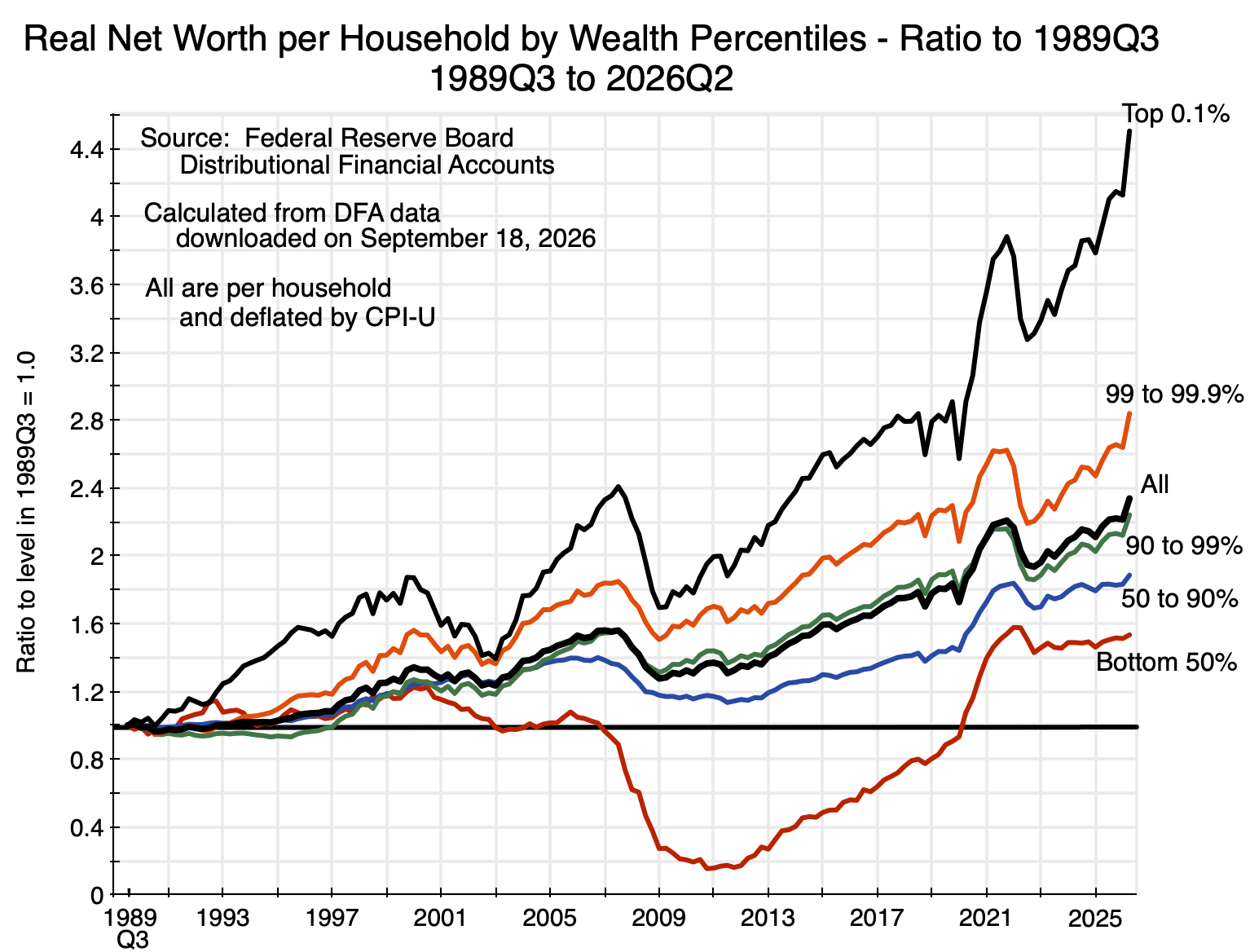
Chart 4

The real net worth per household of the top 0.1% at the end of 2026Q2 grew to be 4.5 times what it was at the end of 1989Q3.  That of those in the 99.0 to 99.9% stratum was 2.8 times as high.  And so on to the bottom 50%, where it was 1.53 times as high.  The wealthier the group to start, the greater the growth in their wealth over the period.

There was no necessity for this.  Indeed, until around 2005, there were times when the relative growth in the net worth of less wealthy groups grew by more than that of some of the more wealthy groups.  But over extended periods, they did not.

But it is also not terribly surprising.  The more affluent can invest in riskier assets, and over extended periods such assets will generally achieve a higher rate of return.  The returns on riskier assets are subject to greater volatility, but over time their higher growth will win out.  This is aside from advantages the wealthy can engineer for themselves through their advantageous capacity to intervene in political processes and decision-making.

E.  Decomposing the Growth in Overall Wealth

The average real value of wealth per household in the US as a whole has gone up substantially over this time period.  It is shown as the thick line in black in Chart 4, and is – as one would expect – in the middle of the increases recorded for the various groups.  Overall net worth (in real terms and per household) in 2026Q2 was 2.34 times higher than what it was in 1989Q3.

What accounts for this?  To start, GDP has grown, but as we will see, the value of wealth has grown by far more.  Breaking this down, the rise has been due to a combination of real GDP growth, an increase in the share of GDP going to earnings on assets (profits), and a higher valuation multiple being placed on those earnings.

To start, profits grew as a share of GDP while the share of wages fell:
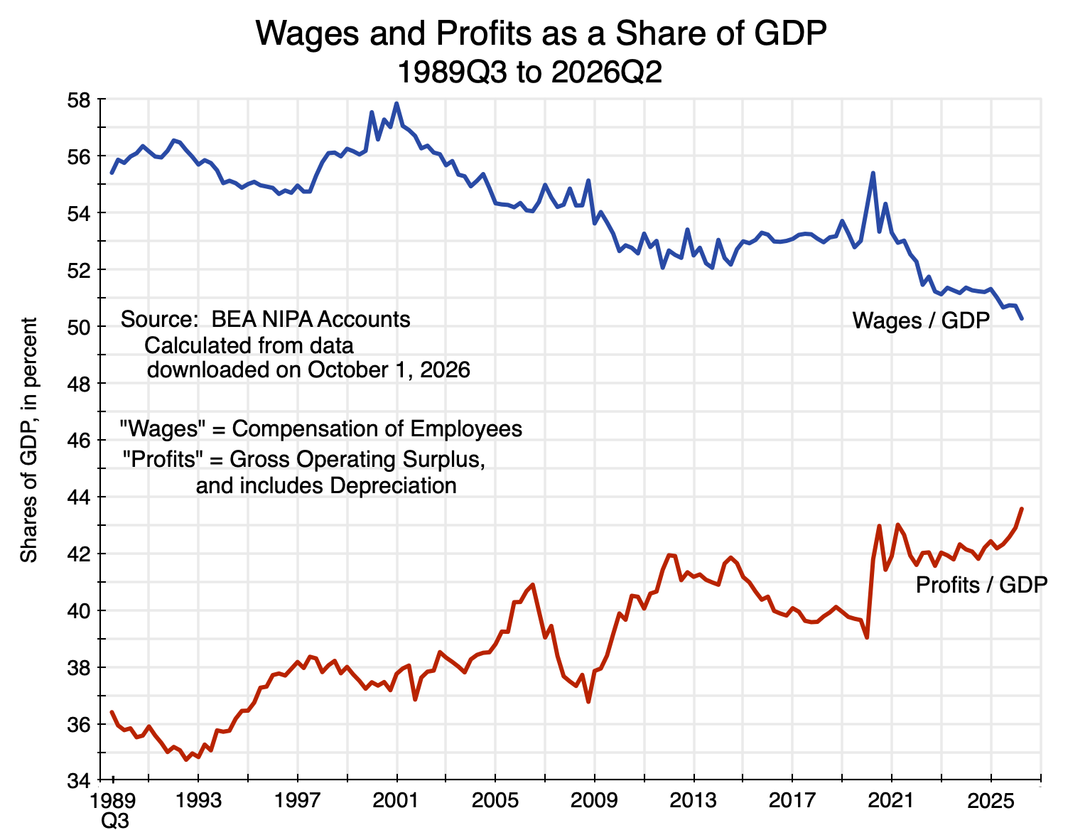
Chart 5

Gross profits (i.e. including depreciation allowances) rose from 36.4% of Gross Domestic Product as of the end of 1989Q2 to 43.6% as of the end of 2026Q2 – an increase (relative to the 36.4% share at the start) of almost 20%.  The share paid to employees (wages) fell from 55.4% of GDP to 50.3%.  As lower income groups are more dependent on wages for their income rather than profits, that fall in the wage share is significant.

[Side note:  The shares of wages plus profits in the chart do not add up to 100% of GDP.  The difference primarily reflects indirect taxes (such as excise taxes on fuels and tobacco, tariffs on imports, state and local property taxes, and more).  Indirect taxes are not counted as being paid out of wages or profits (direct income taxes are), and hence constitute a third category of income in the National Income and Product Accounts.  Those taxes have totaled a steady 6 to 7% of GDP throughout this period (except for a short period in 2020-2021 when they fell with the fall in spending due to Covid), and hence do not affect the trends seen for the wage and profit shares.

There will also be variation in the “statistical discrepancy” – the name the BEA uses for the difference between the estimated values of Gross Domestic Product (GDP) and Gross Domestic Income (GDI).  GDP and GDI should in principle be identical, as the value of all that is produced (GDP) will be someone’s income (GDI).  The statistical discrepancy is small – less than +/- 2% of GDP – but varies over time.  Wages, profits, and indirect taxes are estimated in the GDI accounts, and will sum to 100% of GDI.  But they are expressed here as shares of GDP, which, while close, will not sum to 100% of GDP due to the statistical discrepancy.]

A “valuation multiple” can next be defined as the ratio of wealth (i.e. net worth) for the country as a whole to the profits being earned.  It is akin to a price/earnings ratio often used in valuation measures of equity.  The valuation multiple over this period also rose:
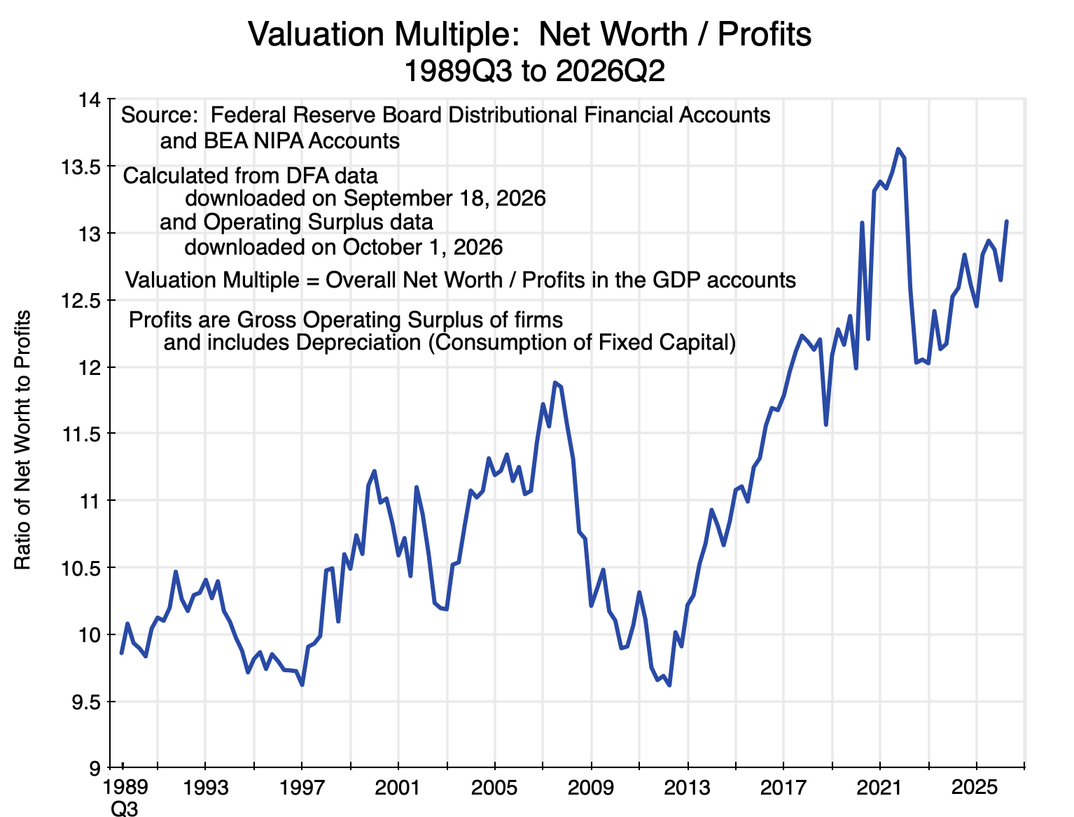
Chart 6

The valuation multiple rose from 9.9 in 1989Q3 to 13.1 in 2026Q2 – an increase of 33%.  But it fluctuated a lot.  It rose to 11.9 in 2007, fell to as low as 9.6 in 2012 following the economic and financial collapse of 2008/2009, and then rose again.  It reached 13.6 in the last quarter of 2021, fell to 12.0 in 2022Q3, and ended at 13.1.

An astute observer might note that the gross profits being assessed here (as a share of GDP in Chart 5, and then as the denominator in the ratio in Chart 6) are the overall profits in the economy.  The corresponding wealth being valued based on those profits is then the wealth held by households.  Will this coincide with the total wealth in the economy as a whole?  The answer is that it will be close, although not exact.  The Fed’s Financial Accounts of the United States (FA), discussed in Section B above, estimates that the aggregate wealth of the US economy as of the end of 2026Q2 was $181.0 trillion (Table S1.b). The Fed’s Distributional Financial Accounts (DFA) estimate the aggregate wealth of households as of the end of 2026Q2 was $185.7 trillion.

These are close to each other but not the same for several reasons.  One is that some of the estimation methods and definitions are different in the DFA accounts than those in the FA accounts, as discussed in Section B above.  But they are close because the ownership of most assets and liabilities is ultimately attributed to households in the DFA.  Households may hold assets directly (such as homes), or via their ownership of equity in both corporate and non-corporate businesses, or their ownership of financial assets (e.g. deposits in banks, or direct ownership of bonds).  These account for most assets in the economy.

The main exception will be government assets – including federal, state, and local government assets.  These totaled $23.1 trillion as of the end of 2026Q2 in the FA accounts.  But largely offsetting this is the net claims on US assets by foreign entities.  These totalled $20.7 trillion, leaving a small net difference.  Coupled with definitional and estimation differences, the total net worth of all US households is reasonably close to the net assets of the economy as a whole and adequate for the purposes here.

Putting this together:  GDP per household rose in real terms, profits rose as a share of GDP, and the valuation multiple assigned to those profits also rose:
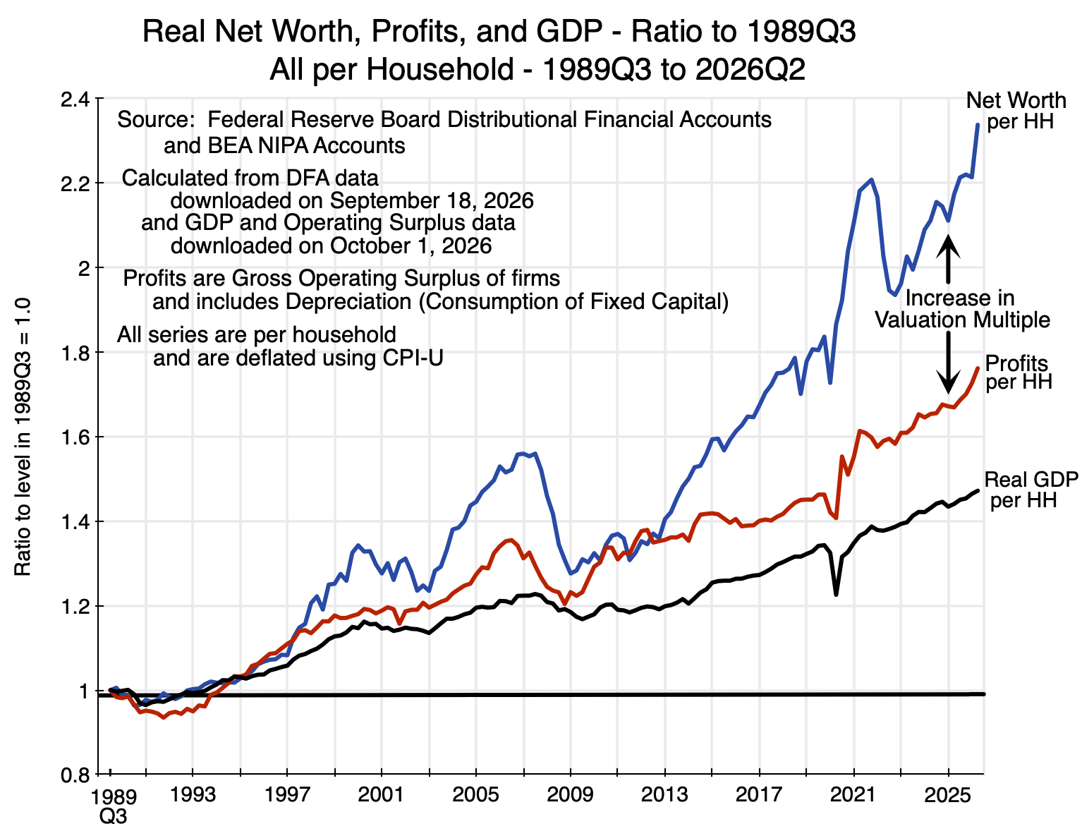
Chart 7

Putting numbers on this, real GDP per household rose by 47.2% over the period, profits as a share of GDP rose by 19.7%, and the valuation multiple rose by 32.7%.  Multiplying this out, the result is:  1.472 x 1.197 x 1.327 = 2.338.  That is, as of 2026Q2, overall real net worth per household rose to 2.338 times what it was in 1989Q3.  That corresponds to the line in blue in Chart 7, as well as the identical line for households as a whole in Chart 4 above (the thick black line).

Decomposed in this way, one sees that the increase in real GDP per household was the largest single factor behind the increase in overall wealth (with its increase of 47.2%).  The economy is producing more now than before.  The increase in the valuation multiple (by 32.7%) was the second most important factor.  Higher valuations are being assigned to assets for any given level of current profits.  And these were then amplified by profits growing as a share of GDP (by 19.7%).  All three were significant, and together led to wealth that is now valued at 2.338 times (i.e. 133.8% higher than) what it was in 1989Q3.

In stable conditions, one would expect wealth to grow in line with the growth in GDP.  But it increased by substantially more over the past 37 years because an increasing share of the income being generated in the economy (GDP) is going to profits rather than wages, and because the value being placed on the assets for a given level of profits (the valuation multiple) has also increased.  Together, they led to an increase in the value placed on that wealth for any given level of GDP by almost 59% (since 1.197 x 1.327 = 1.588).  A good question is why, but that is a topic for a separate discussion.

F.  Conclusion

Overall real wealth per household has grown significantly over the almost 37 years covered by this data series.  Adjusting for inflation using the CPI, it is now 2.338 times what it was at the start in 1989Q3.

But its distribution is highly skewed.  Ranking households by their net worth, the average net worth of the bottom 50% of households was an estimated $63,300 as of 2026Q2.  The average in the 50 to 90% group was an estimated $988,200.  In contrast, the average net worth of the top 0.1% was an estimated $203.7 million, and that in the 99.0 to 99.9% range was $26.7 million.

The disparities were already huge in 1989Q3 – the earliest period in this data series.  But those disparities then grew, with the estimated real net worth per household of the top 0.1% growing to 4.5 times what it was at the start, and that of the 99.0 to 99.9% growing to 2.8 times what it was at the start.  In contrast, while the real net worth per household of the bottom 50% grew, it grew to just 1.53 times what it was at the start.  It also fluctuated widely, and for 13 years (from 2007 to 2020) was less than what it was in 1989Q3.  This was primarily due to depressed values for their net real estate assets.  The value of those assets collapsed in 2007/08, remained depressed for several years, and recovered only slowly.  And real estate accounts for a high share of the net worth of the bottom 50%.

The purpose of this post has been to provide some of the basic figures on the distribution of wealth in the US and to describe how the underlying basic data were estimated by the Fed.  Future posts will examine other aspects of the distribution of wealth, including its distribution when groups are classified by income rather than their wealth holdings, and how wealth accumulation has changed across generations.  A final post will discuss what might be done to address these disparities.
The Fed Faces the Trump Bump in Inflation

Chart 1

The BLS released on September 11 its report on inflation as measured by the CPI for the month of August 2026.  Inflation remains elevated.  It led to prices of futures contracts in the financial markets that predict with near certainty that the Fed will raise short-term interest rates by a quarter point at its upcoming September 15 and 16 Board meeting (technically of the Fed’s Open Market Committee, but often simply referred to as the Board).  The implicit probability of a quarter-point increase – as reflected in the prices of the contracts traded – was 87.3% as of the end of trading on Friday, September 11.

The implications are interesting.  Should the Fed decide not to raise its target rate by a quarter point, the financial markets will be surprised and may react violently.  But should the Fed decide to raise its target rate by a quarter point, Trump may react violently.  And the recently appointed chairman of the Fed, Kevin Warsh, will be in the middle.

Furthermore, there could be significant implications for the upcoming midterm elections, which will be less than seven weeks away.  An increase in interest rates will confirm for voters that inflation is indeed of concern.  But failure to raise interest rates may be interpreted as the Fed caving into political pressure from Trump.  And the next meeting of the is scheduled for October 27 and 28.  An increase in interest rates at that point – should it become blindingly obvious by then that such is needed – would be less than a week before the election.

There are good arguments for why the Fed should raise interest rates now.  Inflation remains elevated well above its 2% target.  The European Central Bank raised its key policy rate by a quarter point on September 10, and the Bank of Japan (which already raised its policy rate by a quarter point in June) is expected to raise its rate by another quarter point next week.

But the August inflation report gives opponents of a rate increase room to argue otherwise.  It basically shows inflation continuing at the rate it has been at for some months now.  That rate is elevated, certainly, and the counter-argument would be that, with it becoming clear that inflation will not fall on its own, the Fed should not continue to delay in the hope that inflation will come down on its own.

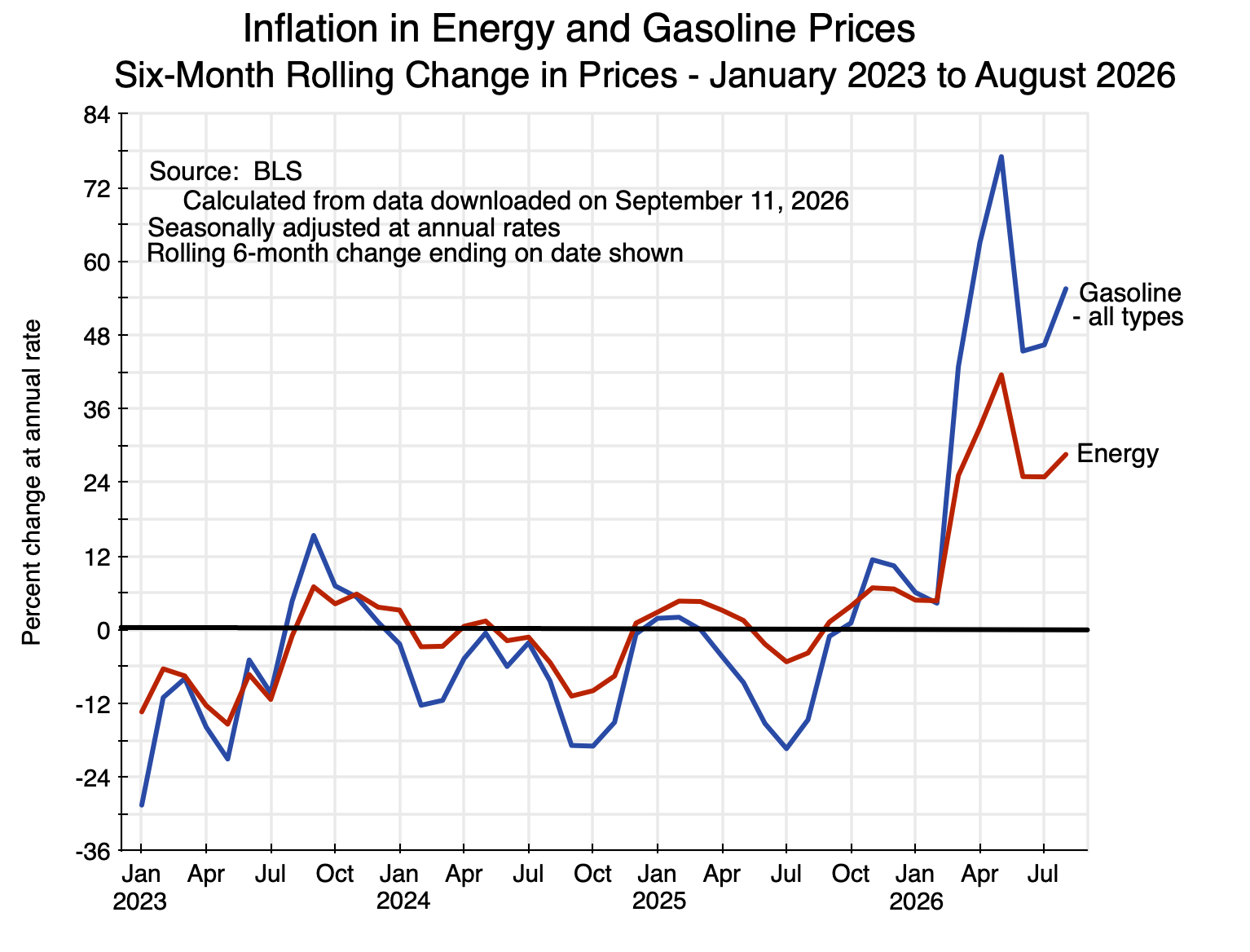
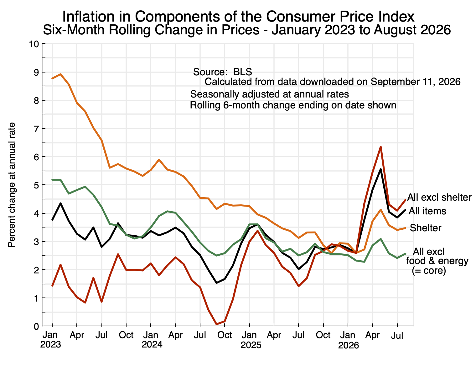
The chart at the top of this post shows the path inflation has taken since January 2023, using six-month rolling average rates to smooth out month-to-month volatility.  The rates shown are for the six-month periods ending on the dates shown, for the overall CPI index, for the core index (i.e. excluding food and energy), for shelter only, and for the overall index excluding shelter.  The rates jumped when Trump started his war against Iran on February 28, 2026, although they had already started to rise more modestly in late 2025.  Interestingly, the price of shelter (as measured in the CPI index) also rose significantly starting in the six-month period ending in April 2026.

Not surprisingly, the increase in energy prices led the way following the start of the war:

Chart 2

This is on a separate chart as the vertical scale would otherwise be so large it would be difficult to follow the changes in the overall inflation indices.  Energy includes all forms of energy – including electricity – purchased by households, including not only fuels for their vehicles but also for heating and cooling their home as well as other purposes.  Gasoline is a sub-component of the overall index for energy.

Note also that these are all seasonally adjusted figures.  The Energy Information Agency (EIA) provides figures on the actual average retail prices (i.e. not seasonally adjusted) of gasoline and other fuels.  The BLS uses these as the basis for its CPI estimates.  The average price for all grades of gasoline sold nationwide in mid-February was $3.057 per gallon.  It rose to $4.182 as of mid-August.  The inflation figures reported by the BLS are for the prices as of the middle of each month (the week that includes the 15th of the month).

The overall CPI inflation rate remained elevated, at 4.1% as of the six-month period ending in August.  This is well above the rate of 2 1/2 to 3% for most of mid to late 2025.  But note that the core rate of inflation – i.e. inflation for all items other than food and energy – has been around 2 1/2% for the six-month periods ending in June, July, and August.  That rate is also similar to what it was in most of 2025.  While still above the 2.0% target, inflation of 2.5% is a lot closer to that target than a rate of over 4%.

This should not be taken – in my view – as meaning inflation is not a concern.  Inflation as measured by the core price index for Personal Consumption Expenditures (PCE) in the GDP accounts has been substantially higher.  The Fed prefers to focus on that estimate as a measure of inflation over the core CPI.  The figures (through June) were discussed in the prior post on this blog.  The August estimate will not be released until September 30, but inflation in the core PCE price index was 3.5% for the six months ending in July.  That is well above the 2.5% rate for the core CPI.

Still, the Fed Board has the CPI estimates for August and does not yet have the PCE price indices.  If Kevin Warsh wants to argue interest rates should not be raised, he could focus on the core CPI figures as a rationale, saying they do not show inflation to be excessively high.

This could present an opening for a decision by the Fed to leave its target interest rate unchanged.  If it does, then as noted above, the financial markets might react violently, as this would be a major surprise given the strong expectation (reflected in the price that futures contracts are trading at) that the Fed’s interest rate target will be raised.

We will see what happens on September 16.  The Fed will announce its decision at 2:00 pm ET.

===============================================================

Update on September 16, afternoon:

As expected by the markets, the Fed raised its short-term interest rate target by a quarter of a percentage point.  The initial market reaction was neutral (the increase was as expected), but then declined modestly while Fed Chair Kevin Warsh held his post-meeting news conference and made clear that inflation is indeed of concern – and perhaps more of a concern than the markets realize.

Trump also responded as expected:  he was mad.  At 4:38 pm he posted on his social media site “Truth Social”:

Interest Rates in the United States should be 1%, or less, because we are the Best Credit in the World — BY FAR. Our Country is BOOMING with new Investment! If we stopped Trading with every country that we have a Deficit with, which is most of them, we would make, at least, 1.5 Trillion Dollars a year. The word “Deficit” is nothing more than a fancy word for LOSS. We are “carrying” almost every country in the World, and that cannot go on any longer. LOWER THE INTEREST RATES FOR THE UNITED STATES OF AMERICA, AND FAST! President DONALD J. TRUMP

It is another sign that the president of the United States is completely unhinged, with no understanding of basic economics.

Weakening Growth and Signs of Overheating: The US Economy Under Trump

Chart 1

A.  Introduction

Economic growth has weakened under Trump, with GDP growth falling to below 2% at an annual rate in the year and a half since he took office.  GDP grew at a rate of close to 3% in the last year and a half of Biden’s term in office.  Furthermore and importantly, much of the GDP growth during Trump’s second term can be attributed to the sharp increase in investments in equipment for information processing and related items – the AI boom.

While the import content of AI-linked investments is significant, one can get a sense of the direct impact on GDP of those investments under reasonable assumptions.  As will be discussed below, the growth in GDP other than production for AI-linked fixed investments has been less than 0.9% at an annual rate during Trump’s second term, when account is taken of the estimated import content of that investment.  It would be less than 0.7% if the import content of AI-linked investment is ignored (as many do).

This poor record should not be surprising.  Trump has enacted numerous policies – often hastily – that critics have noted would harm growth.  They have.  Section G below will briefly discuss some of the more prominent among them.  But the primary focus of this post will be on the data, and in particular on data now available with the release on July 30 of the initial estimates from the BEA of the NIPA (i.e. GDP) accounts for the second quarter of 2026.

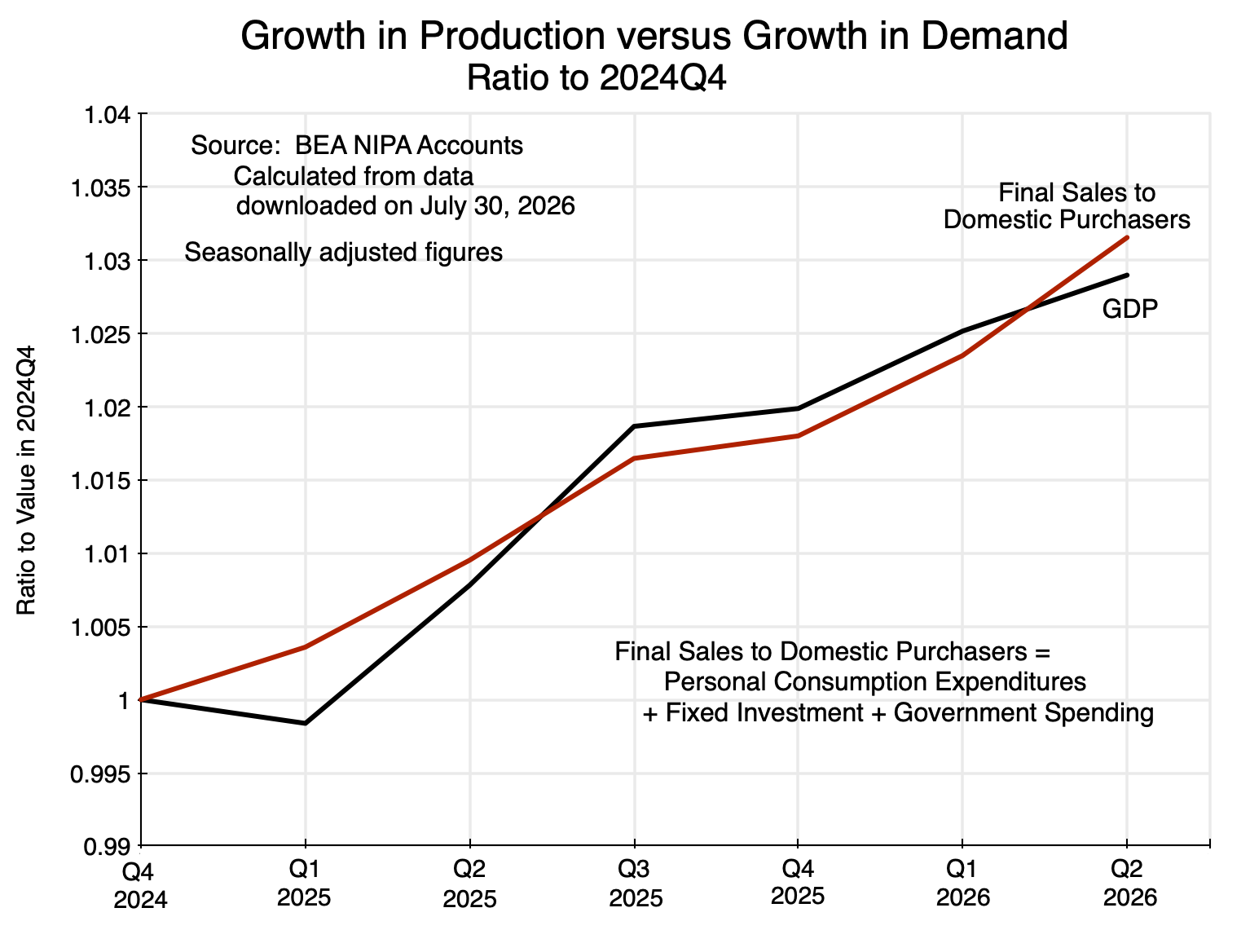
The GDP figures for the second quarter are also of interest as they show what happens when domestic demand grows more rapidly than the limits of what domestic supply can provide as capacity limits are reached.  GDP is a measure of supply, i.e. of domestic production (which is why it is called Gross Domestic Product).  It grew at an annual rate of just 1.5% in real terms in the second quarter.  But domestic demand grew substantially faster.  Final sales to domestic purchasers grew at a rate of 3.1%.  These final sales are the sales for personal consumption, for fixed investment, and for government spending on goods and services, and could grow faster than supply only because the trade deficit increased and inventories were drawn down.  That is, sales came from greater imports and out of inventories that had been produced in the past.

With unemployment low (at a 4.1% rate in July – higher than under Biden but still low by historical standards), the economy was not able to produce much more despite the increase in demand.  A slowing economy while demand is growing faster is a recipe for overheating.  And there are indications that inflation is indeed rising as a consequence, even aside from the compounding factor of the higher energy prices resulting from Trump’s decision to start a war with Iran.

Section B will first look at what has happened to growth in GDP in the first year and a half of Trump’s second term, with this compared to what it was in the last year and a half of Biden’s term.  It has slowed substantially, from growth at a 3% pace under Biden to below a 2% pace now.  Furthermore, and as noted above, much of this growth can be attributed to fixed investments related to the AI boom.  Growth in everything other than production for the AI boom has slowed by substantially more.

Why did growth in GDP (i.e. growth in production) slow?  Section C of this post will start to address this by examining what has happened to fixed investment under Trump.  While AI-related investment has boomed, fixed investment in everything but the AI-related investments has gone down in absolute terms during Trump’s term.  Instead of growing – as a healthy economy needs – such investment is now 8% below where it was in the fourth quarter of 2024 – the last full quarter of Biden’s term.  This affects the supply of capital.

Section D will then look at the growth – and recent decline – in the labor force.  The labor force is shrinking under Trump in contrast to modest growth under Biden.  Trump’s aggressive policies to deport migrant workers have been an important factor behind this.

Section E looks at the balance between aggregate supply (GDP) and aggregate domestic demand (Final Sales to Domestic Purchasers).  The difference is the trade balance and the net change in inventories.  The more rapid growth in domestic demand in the second quarter of 2026 than the growth in domestic supply had to be met by a larger trade deficit (higher imports) and a drawdown of inventories.  This is a sign of an economy that is overheating.  Inventories can only be drawn down to the extent there are inventories to draw from; it cannot continue forever.  And while a trade deficit can be sustained as long as foreign lenders are willing to fund it (and the US has had a significant trade deficit since the mid-1980s – they began under Reagan), the increase in the deficit is a sign of an economy reaching the limit of what it could produce domestically during the period.

This is an early sign of an economy that is overheating, due here to a combination of rapid domestic demand growth with a weakening of the economy’s ability to supply that demand.  It is also directly counter to Trump’s claims that his tariff policies will lead to a sharp reduction in the trade deficit (as well as a stronger economy, he asserts).  He has the economics of this wrong, and the consequences are clear in the data.

An overheating economy is reflected in the inflation numbers.  These are reviewed in Section F of this post.  Inflation is now rising, and the turning point on this began already in the fall of 2025, well before the war on Iran was launched.  The war then led to a sharp rise in energy and certain other prices, which has compounded the underlying problem.  This has resulted in real wages falling.  Living standards for most have diminished, with Disposable Personal Income faltering already in late 2025 and falling in 2026.

Why has growth in GDP weakened?  Section G of the post will list a few of the policies under Trump that have hurt growth.  Section H will present some scenarios of what might happen now, and Section I will conclude.

B.  Growth in GDP

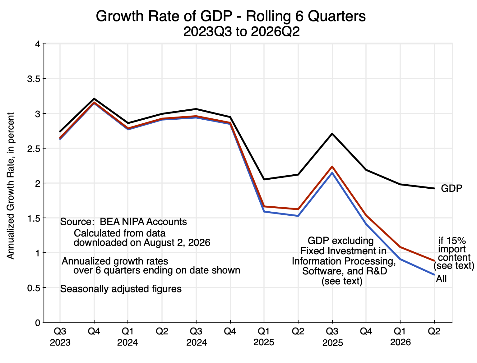
GDP growth has weakened.  While there is substantial volatility in the quarter-to-quarter changes, a rolling average over six quarters will smooth those out to show the trends.  Growth (at annual rates) fell from about 3% during the later years of Biden’s term in office to less than 2% during the first year and a half of Trump’s second term.  See the chart at the top of this post.

Furthermore, much of that 2% growth was driven by the boom in AI-related investments.  The entire rest of the economy has been growing even more slowly.  Based on a reasonable estimate of the growth resulting from production to support the boom in AI-linked investments, the rest of the economy has been growing at a rate of below 0.9%.

To clarify a point of possible confusion:  The 0.9% growth rate refers to growth in the supply of production for everything included in GDP other than production for the AI-linked investments.  The estimate of the impact of the AI-linked investments does not refer here to growth that might result from the demand-side impact on GDP of such investments.  An increase in investment can spur GDP growth by increasing consumer and other demands for output in the standard Keynesian way in times when unemployment is high and production is constrained by aggregate demand.  But production is not now demand constrained (as will be discussed in Section E below) while unemployment (at 4.1% in July) is low by historical standards.

The question being addressed here is the growth of all that is included in GDP other than production for the AI-linked investments.  That figure is a better estimate of the impact Trump has had on economic growth than the growth in overall GDP.  The AI boom is a consequence of developments that have been underway over a decade or more, and are now materializing in massive investments for data centers and related items to support the further development of the AI models and to make available their services.

The National Income and Product Accounts (NIPA, often loosely referred to as the GDP accounts) do not specifically provide line item figures for investments dedicated specifically to the provision of AI services.  This is, of course, not surprising; AI is new.  However, the NIPA accounts do provide estimates for fixed investment in equipment for information processing purposes, as well as for investment in software and in research and development (R&D).  While there have long been such investments, much of the increase in such investments since early 2025 is likely due to investments that are linked to what was needed to support the new AI systems.

This will nevertheless likely overestimate the investments just for AI, as there will be new investments in those categories for purposes other than AI.  Acting in the other direction, the line items shown in the NIPA accounts are solely for equipment produced for such investments (plus investment in software and R&D).  AI-linked investments will also include investments in structures, which are a separate category in the NIPA accounts.  There are also supporting investments in areas such as new power generation capacity (AI is creating a huge demand for additional power), new water systems, fiber optic cable networks to connect them all, and more.

Treating the investments in information processing equipment, software, and R&D as “AI-linked” investments is therefore a shortcut and certainly imperfect.  But it will suffice for the purposes here, which is to give a sense of the extent to which the growth in GDP has been due to such investment, and how limited growth has been outside of that narrow area.

An additional difficulty is that the figures on investment and the other items in the GDP accounts do not (and cannot) show to what extent imports are a source of supply (directly or indirectly) for those expenditures.  Imports are taken into account for overall GDP by simply adding up all of the demands (i.e. for consumption, total investment including in inventories, government spending, and exports) and then subtracting total imports.  But it is impossible to come up with good estimates of the extent to which imports accounted for the supply of the items that were used to satisfy some specific demand, especially in some indirect way.  One knows, for example, how much fuel was imported in total to supplement the domestic supply of fuels, but it is impossible to know how much of the fuel used directly and especially indirectly to produce some specific item was imported rather than domestically supplied.

We do know, however, that a substantial share of the expenditures to build the new data centers are imported.  The semiconductor chips required are almost all imported (from Taiwan for processors and Korea for memories), as is a substantial share of the specialized equipment.  But the cost to build a new data center is more than just the cost of the chips.  Furthermore, one should not count the gross cost of an imported semiconductor chip used in such centers.  Much of that cost goes back to the American firms that designed them.  Nvidia – the source of the graphical processing unit chips used in the data centers – enjoys a gross margin of 75%.  That means that of $100 in revenues from its sales of chips and other products, the cost to it of the goods it sold (e.g. what it paid to TSMC in Taiwan to fabricate the chips, which were then imported) was just $25.  The gross cost of the chips imported will be $100, but $75 of this is earned by Nvidia to cover its costs to design the chips and as profits accruing to it as an American firm.  Taking this into account, the net import cost was only $25, not the value at the “list price” of $100.

Furthermore, while a significant share of the cost of building the AI data centers is accounted for by imports, there has also been a substantial increase in related investments in the production of software and in R&D.  Imports do not play a major role in the production of either of these.  Together, they accounted for 70% of the investment that increased sharply in the AI boom.  Investment in “Information Processing Equipment” was just 30% of the total.

Thus, assuming (probably on the high side) that 50% of the cost of the investment in new data centers (the Information Processing Equipment) comes from imports, and essentially no imports for the 70% accounted for by the investments in software and R&D, the import share of what was invested as a result of the AI boom would be 15%.  That is, 85% of the cost would be domestically supplied.

The chart at the top of this post shows total GDP growth during this period, and then the growth in GDP for everything other than what was produced for the investments going into the AI boom.  Based on the estimate of a 15% import content in the production of what was invested in the AI-linked investments, the growth in GDP in everything other than for the AI investments has been at an annual rate of less than 0.9% during Trump’s term in office so far.  Ignoring the import content (and thus implicitly setting it at zero), the growth rate would have been less than 0.7%.  Either is a substantial fall from the approximately 3% rate under Biden.

Furthermore, despite its recent rapid growth, domestic production for the investments in information processing equipment, software, and R&D only accounted for 8% of GDP in the second quarter of 2026.  That is, the “rest of the economy” is 92% of GDP.  This 92% of GDP has grown at a rate of only 0.9% since Trump began his current term in office.

Why this fall in growth?  Supply comes from production using capital and labor, and both are declining.

C.  Fixed Investment

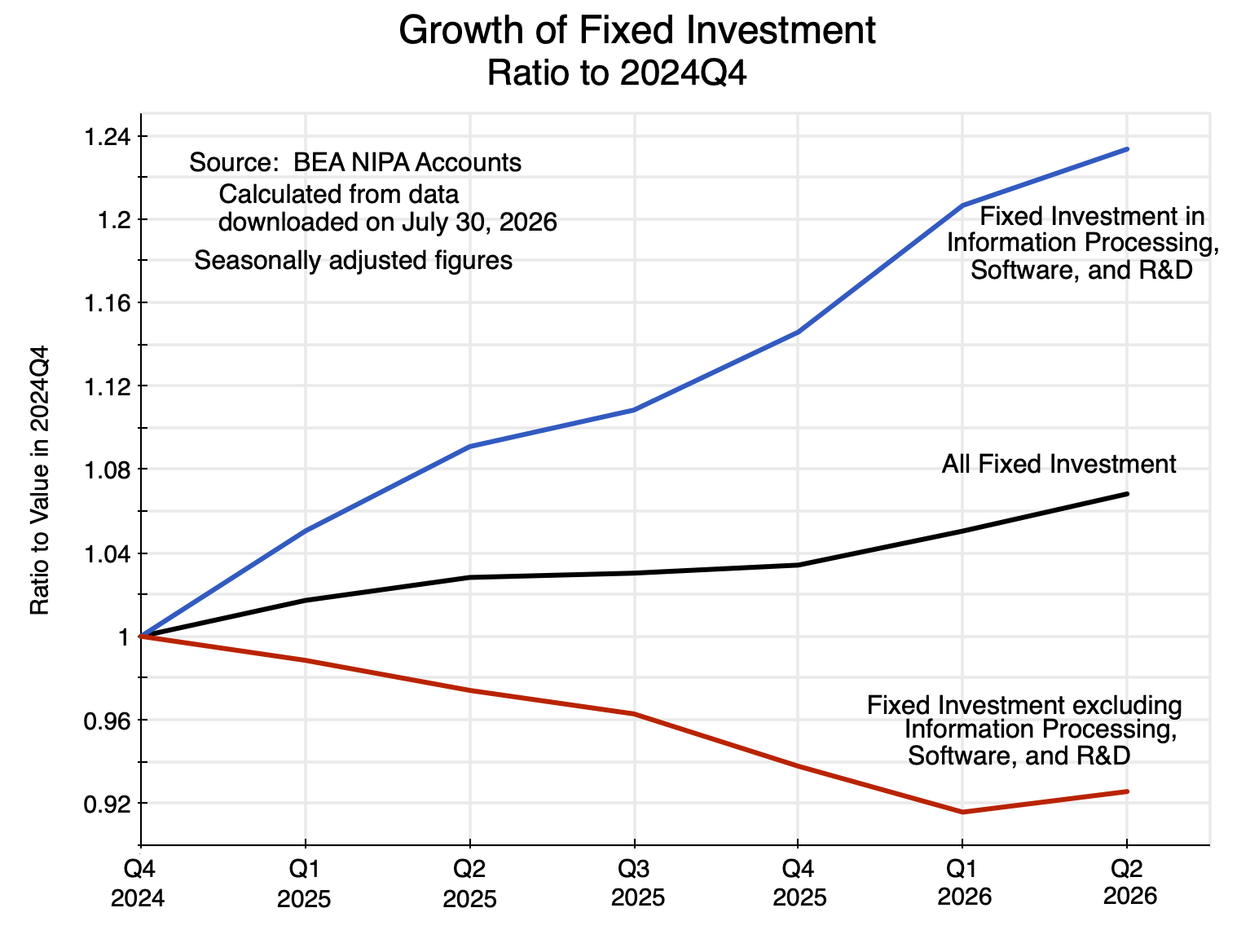
Capital is produced by new fixed investment.  While overall fixed investment has grown by a total of almost 7% over the year and a half in Trump’s second term (4.5% at an annual rate), all of the growth was due to the rapid growth in investments for the AI boom.  Those rose by over 23% during that period (15.0% at an annual rate).  Fixed investment in everything else in the economy actually fell by 7.4% (a fall of 5.0% at an annual rate):

Chart 2

Other than the investments in the items linked to developing and providing the new AI services, investment has performed poorly under Trump – indeed terribly.  Investment in residential structures (housing) fell in every quarter but one during this year and a half, and by the second quarter of this year was 5.3% below where it was in the last quarter of Biden’s term in office.  Investment in nonresidential structures (i.e. commercial real estate, offices, warehouses, factories, etc.) was even worse:  It fell in every quarter since Trump returned to office, and is now almost 8% below where it was at the end of Biden’s term.  All other investment items (primarily other equipment) fell in three of the six quarters and rose in three, and ended up at just 0.95% above where it was under Biden.

The result is that the supply of capital for all of the economy other than for providing AI services is now well less than what it would have been had investment been sustained as it had under Biden.  Over 2023 and 2024, total fixed investment grew at an annual rate of 3.3% while investment in all but the AI-linked investments grew at a 3.0% rate.  These supported and were consistent with GDP growth during the period of about 3%.  Under Trump, investment other than for AI fell.

D.  Labor Force

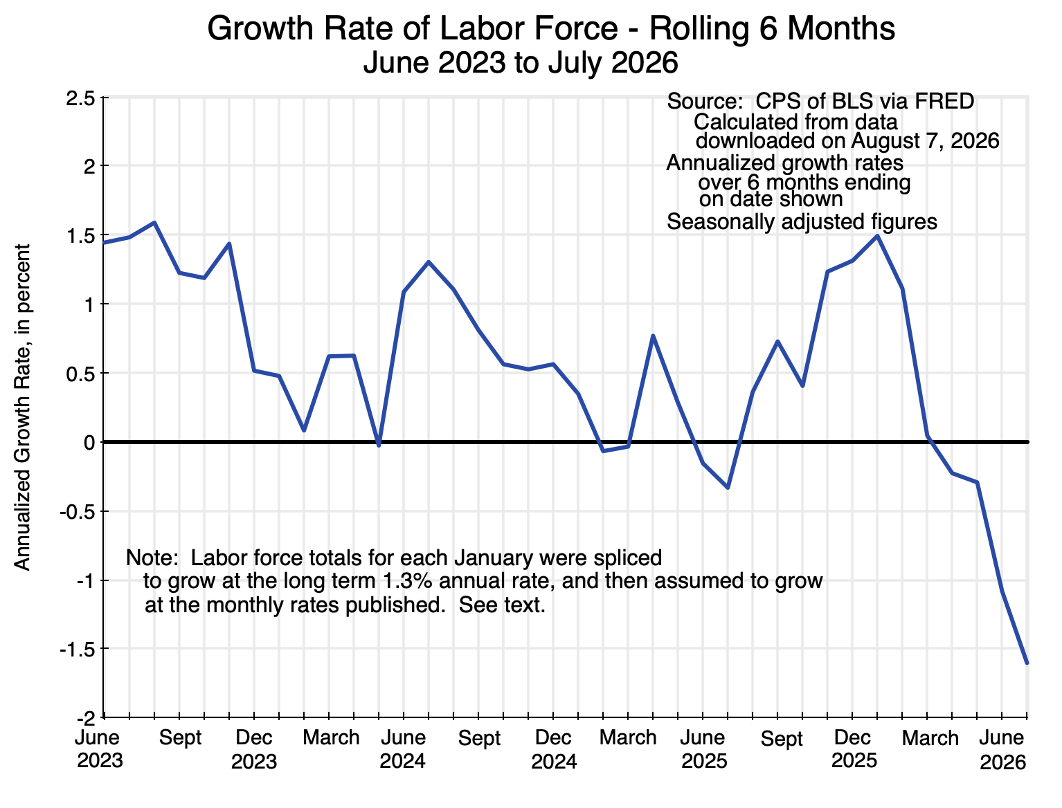
Labor is the other source of supply.  And there is now less of it to support the American economy:

Chart 3

The chart shows the estimated growth in the total labor force in the US on a rolling 6-month basis.  A person is considered to be in the labor force if they are employed or, if unemployed, have been actively looking for work at some point during the four weeks leading up to and including the week of the survey.

Comparisons over time of labor force statistics are, however, complicated by the fact that they derive from figures in the Current Population Survey (CPS) of households of the BLS.  The issue is that the population weights used to derive US-wide estimates from the set of households surveyed are updated every January.  But the BLS does not then go back and revise the estimates issued before.  Thus there will always be a “jump” in the estimates (up or down) in the January figures from those of December.  That means one cannot properly estimate growth rates for the labor force for periods that straddle December to January (although many analysts ignore the issue and do it anyway).

This is in contrast to the approach taken in the Current Employment Statistics Survey (CES) of the BLS – its survey of business establishments (both public and private) from which it derives estimates of total non-farm employment.  Those employment estimates are updated on a regular annual cycle to produce figures that are comparable across time.

For Chart 3 above on the labor force,  I adjusted the CPS data by in essence splicing the series in each January from 2022 onwards by assuming the growth in the labor force in that month was simply the long-term rate of growth between December 2022 and December 2025.  That rate was 1.30% (in annual terms).  The growth in the labor force in every other month but January was as recorded in the CPS data.  This smoothed the series by removing the jumps each January and substituting for that month – and that month only – the overall rate of growth since December 2022.  Without the splicing in this manner, the jump in the labor force estimates would have been up in two of the four years and down in two of the years.  The spliced series provides a better sense of the trends in the size of the labor force, and will suffice for the purposes here.

Furthermore, keep in mind that the six-month growth rate for the period ending in July 2026 is the growth rate from January to July.  That period is not affected by whatever adjustment was made to smooth out the December to January jump when new population weights were introduced.  And from January to July of this year the total labor force fell at an annual rate of 1.6%, consistent with the trend seen in the chart for the prior months.

A declining labor force has significant implications for how fast GDP can grow.  Without additional labor, GDP can grow only as fast as productivity does, and that is limited.  Since the start of Trump’s second term in office, labor productivity (the ratio of GDP to workers employed) has on average grown at an annual rate of 1.6% – down some from the 1.9% rate in the final year and a half of Biden’s term.  If the labor force is falling at a rate of 1.6% a year – as it is now – then at a 1.6% rate of productivity growth, GDP will not grow at all.  And if one assumes the labor force will now stop falling and remain flat, GDP could grow at only a 1.6% rate if that rate of productivity growth is sustained.  That is still about half the rate of growth in GDP achieved in the last year and a half of Biden’s term (and also half of what it was in Biden’s full term).

It is not surprising that there has been a sizable fall in the size of the overall labor force this year.  The Trump administration has moved aggressively against migrant workers, incarcerating and deporting many.  Of those not detained, many have withdrawn from the labor force in order to keep a lower profile.  And the actions taken against migrants are not only against those who have not been given official status.  Roughly three-quarters of the migrant population in the US has legal status.  However, the Trump administration has sharply curtailed the number of new applicants they are approving for some form of legal status, while also removing or curtailing the legal status of many who had had it before (such as those with asylum or refugee status).  All of these actions have led to a reduction in the number of workers in the labor force.

This is coming on top of the aging of the native-born population, with an increasing share moving into their normal retirement years.  The consequence of this demographic shift is that while the native-born adult population has been growing at a rate of between 0.7 and 0.8% per year (calculated over a period starting before the Covid disruptions, when there were sharp fluctuations in the recorded data), the labor force of the native born population has been growing at a rate of just half that – between 0.3 and 0.4% per year (based on BLS data).  That rate is expected to fall further in the coming years.  Workers are needed, and Trump is deporting them.

Migrant workers contribute to the economy.  The value of their work in a market system (and as measured in the GDP accounts) is greater than what is paid to them in wages.  Furthermore, removing them from their jobs has not led to a reduction in unemployment of native-born workers.  That is, the jobs they had are not now being taken up by previously unemployed native-born labor.  Their unemployment rate as of July, while low at 4.6% for the native-born population and 4.1% overall, was lower under Biden.  Removing migrant workers has led to a smaller labor force and thus the contribution they make to the economy.

E.  Demand is Growing Faster Than Supply

GDP growth, as discussed above, has weakened significantly under Trump.  GDP is a measure of domestic production (i.e. supply).  While often measured through the demand components of GDP (since what is produced will be sold, once one takes into account changes in inventory levels), GDP is not itself equal to demand.

One can, however, easily arrive at a measure of aggregate demand by adding up the estimates for Personal Consumption Expenditures (expenditures by households on consumption items), for Private Fixed Investment, and for Government Spending on goods and services.  This is known as “Final Sales to Domestic Purchasers” and differs from GDP in that it leaves out changes in inventories (hence the use of the term “Final”) and also the trade balance (i.e. Net Exports, or Exports minus Imports, and hence the term “Domestic Purchasers”).  A drawdown of inventories will add to the flow of supply produced domestically in the period, as will the net amount obtained through the trade deficit (with an increase in net supply by exporting less or importing more).

Expansions in aggregate demand can lead to an expansion in domestic supply in the standard Keynesian way when there is available extra capacity to produce those goods and services as well as labor that can be hired.  But there are limits to what can be produced domestically, including limits on how much labor can be newly hired when an economy is at or close to full employment.  At times such as those, an increase in aggregate demand will not be met by a similar increase in aggregate domestic supply, but rather by increased pressure to draw down inventories and to run a larger trade deficit by exporting less and especially (and usually) by importing more.

This is what was observed in the accounts for the most recent quarter.  Final Sales to Domestic Purchasers rose at a 3.1% rate, but domestic supply (GDP) could not keep up and rose at only a 1.5% rate:

Chart 4

The chart shows the increases in demand (Final Sales to Domestic Purchasers) and domestic supply (GDP) – all in real terms – during Trump’s current term in office.  They will normally move roughly in parallel.  The fall in GDP in the first quarter ot 2025 was mostly due to the anticipation that Trump would soon be charging high tariffs on imports (which he did), leading firms to accelerate their purchases of imports to get ahead of the anticipated tariffs (with a resulting major increase in the trade deficit in the period), along with a cut back in purchases from domestic suppliers to balance this.

Note, however, that while the curves in the chart cross in the second quarter of 2026, no special significance should be assigned to that fact alone.  They are both drawn relative to their levels in the fourth quarter of 2024, and there was already a trade deficit in that period.  Indeed, the US has run significant trade deficits since the 1980s when, under Reagan, there were large tax cuts as well as major increases in government spending (primarily for the military).

Rather, the point to note is that the increase in Final Sales to Domestic Purchasers (demand) in the second quarter of this year was significantly greater than the increase in GDP (supply).  To meet that higher demand, the economy had to draw down inventories and run a larger trade deficit.  The relatively weaker growth of GDP (of just 1.5%) is a sign that domestic production could not keep up with the increase in domestic demand.

Not surprisingly, White House officials as well as at least some news reports misinterpreted this and treated the relatively rapid growth in demand as a sign of strength in the economy.  Demand did, indeed, grow.  But supply could not keep up.  That is what happens when an economy starts to overheat.  And when an economy overheats, inflation rises.

F.  Inflation is Rising, and Real Wages and Personal Income Are Falling

Inflation has gone up this year, driven in part by the high oil and gas prices resulting from Trump’s decision to start a war against Iran.  But inflation in fact started to rise last fall, well before the attacks against Iran were launched on February 28.

Inflation rates over rolling six-month periods work well for finding turning points.  There is too much statistical noise in one-month only changes, while changes over twelve months (i.e. year-on-year) are too long before changes in trends are recognized.  Yet most analysts and news reports focus on the one-month and twelve-month changes.

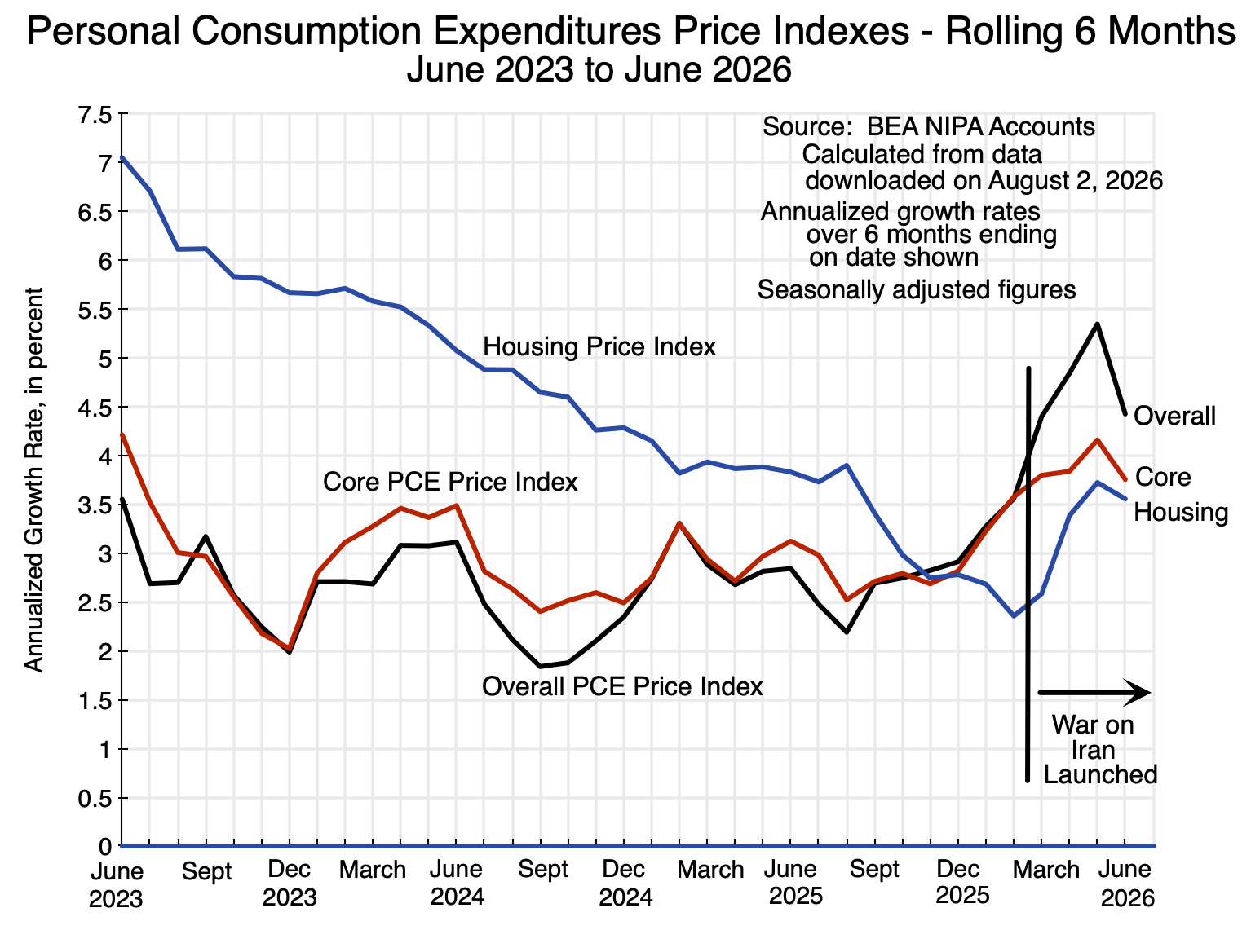
Based on the six-month rolling change in prices, increases in the price indices for Personal Consumption Expenditures (both overall and core, where the core price indices exclude food and energy) were mostly within the range of 2.5 to 3.0% at annual rates through most of 2025 (with a few exceptions on each side).  They were also about that, on average, in the last two years of Biden’s term.  But the rate of increase of both price indices then started to go up in the six-month periods ending in January and especially February 2026.  Note that prices for these indices are recorded as of the middle of each month, so the first set of prices following the February 28 start of the war on Iran are reflected in the March figures:

Chart 5

Note also that inflation in the price index for Housing had been falling steadily from at least 2023.  Housing has a significant weight in the PCE price indices (15% in the overall PCE price index and 17% in the core PCE price index – see the discussion in this earlier post on this blog), so it matters.  But the housing price index also changes with a lag, as it is estimated from surveys of rental households on their cost of renting similar housing.  Rental contracts are typically set in the US for a 12-month period.  Inflation in the price index for Housing, as measured, continued to fall into 2026, and in fact fell below the rates for the overall and core PCE price indices.  This acted to moderate somewhat the rise in those indices in late 2025 and early 2026.  But then inflation in the price index for Housing soon started to rise as well, confirming the general upward pressures seen on prices.

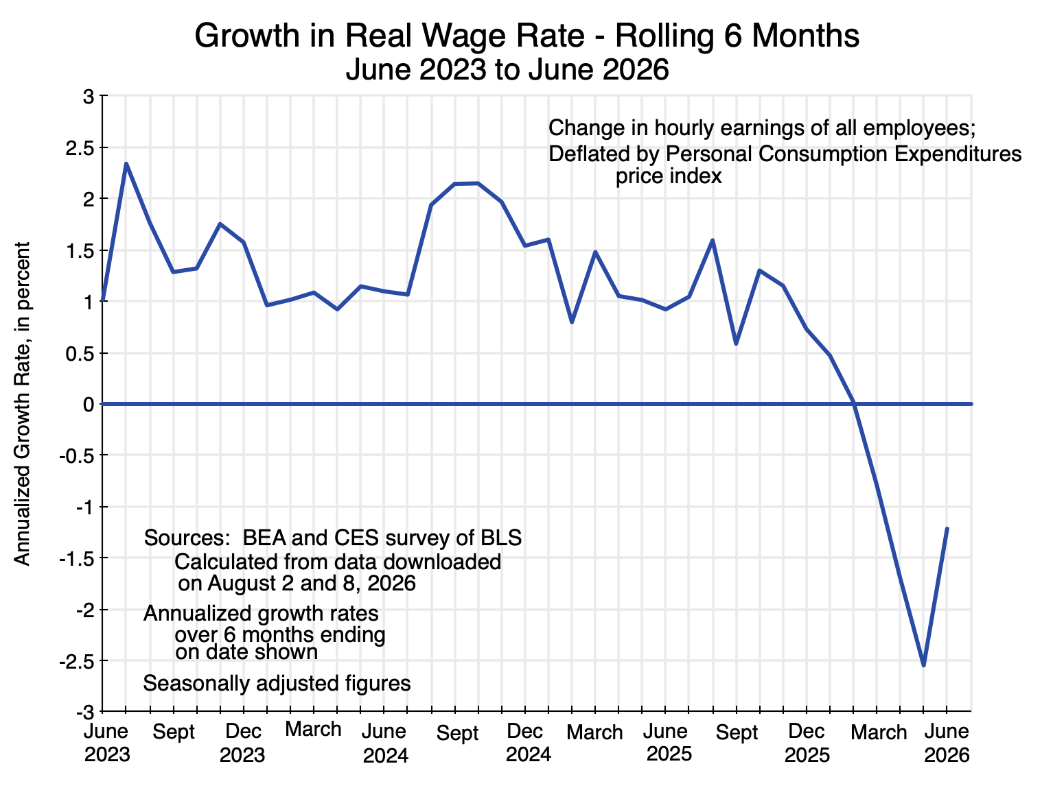
A consequence of the rise in inflation has been a fall in real wages:

Chart 6

Real wages were rising in the last two years of the Biden administration, but in 2026 wages have not kept up with rising prices and have fallen in real terms.  Should wage demands now rise to try to offset this, there is a danger that the economy could end up in a wage-price spiral.

The result has also been a fall in real per capita Disposable Personal Income:

Chart 7

Real Disposable Personal Income had been steadily rising as Biden left office, and continued upward in the early part of Trump’s term.  But it already started to falter in late 2025 (notably before the Iran war had its impact on prices) and is down in 2026.  (Disposable Personal Income is Personal Income after personal taxes are paid and transfers – such as Social Security – are received.  It is deflated in the NIPA accounts by the PCE price index.)

Inflation will increase when an economy is operating at full capacity and full employment, and there is pressure from demand rising by more than supply.  That is consistent with what is observed here.  Demand – at least through the second quarter of 2026 – has grown at a relatively rapid pace.  But supply has not kept up, and is indeed slowing.  Given what Trump has done, that is not surprising.

G.  Trump’s Policies Are Hurting Growth

Why has growth weakened?  The purpose here is not to provide an in-depth analysis, but rather just to summarize a few of the more obvious examples of decisions that have hurt growth and increased costs:

a)  High, arbitrary, and often capricious tariffs have been imposed on essentially everyone, including on imports from nations that had been the closest allies of the US.  Many were announced by Trump in late-night posts on his social media accounts.  Trump also often soon changed them to something else – also often announced via social media.  Not only did they violate international trade treaties that the US had negotiated and approved over decades, many were also clearly illegal under US law.  But it took some months for the cases to wind through the courts to an eventual final decision.

Tariffs have an immediate impact on prices.  They are in essence a sales tax, paid by the American firms importing the items and then passed on (to the extent they can) to American households.  Trump has insisted that foreign exporters are bearing the cost of the tariffs (by reducing the prices they charge by that amount, he asserts), but careful empirical studies of the actual data have found this not to be the case.  While theoretically possible, a recent careful study found that US firms and households are bearing 96% of the cost of Trump’s tariffs.  Other studies have had similar findings.

In addition, with high but variable and uncertain tariffs facing them, firms are in a poor position to plan on how much to invest and in what.  They cannot be sure how much they will be paying in tariffs on what they need to import, nor what price they will be able to charge for what they produce.  It is thus not surprising that investment in everything other than items related to the AI boom has declined under Trump (as seen in Chart 2).

b)  Trump’s aggressive policies against migrant workers have reduced the labor force.  But labor is needed in an economy.  And removing migrants from the labor force has not led to increased employment of native-born workers:  Their unemployment rate – while relatively low (4.6% as of July 2026) – is higher than what it was during Biden’s term.

With less labor, less can be produced.  But what is produced with labor has a value greater than what is paid in wages in a market system (and as measured in the GDP accounts), so the cost is borne not just by those taken away from the workforce.  The result is slower growth.

c)  The war Trump started against Iran on February 28 has also hurt the economy.  It led to increases in the cost of not just oil (crude and refined products), but also items such as natural gas (LNG), petrochemicals, fertilizers and fertilizer components, and other such products due both to direct war damage and to a drastic reduction in shipments through the Strait of Hormuz.  While the US is also a producer of many of these, US firms and households will still pay higher prices for such products (and for the products that these are used as inputs to) as the prices are determined globally for such goods.

d) Trump has also brought in blatant clientelism, where favored firms and friends can benefit greatly while unfavored firms are punished.  There have been several avenues for this.  One has been “donations” by firms to special projects Trump has initiated.  An example is the building of a grandiose new ballroom on the grounds of the White House, where as of last November over 37 firms and individuals had donated $300 million.  There have also been massive amounts raised in various Political Action Committees sponsored by Trump, where already in August 2025 Trump said on his social media platform that over $1.5 billion had been raised since his November 2024 election.  This is unprecedented for a president in his second term.  And there have been numerous examples of direct payments coinciding with favorable treatment in legal cases, presidential pardons, and similar actions by the administration.

Trump and his immediate family have gained unprecedented wealth during his new term in office.  Only rough estimates are possible, however, as Trump has been far less transparent than prior presidents on his finances.  Prior presidents released their tax returns, for example, but Trump has refused.  A minimum estimate is possible based on a mandatory financial disclosure, but that disclosure only provides figures in ranges, such as $5 million to $25 million, $25 million to $50 million, and anything above $50 million.  But based on what was provided in the disclosure, reporters at The New York Times concluded that Trump brought in a minimum of $2.2 billion in 2025.

Firms and wealthy individuals may well feel obliged with this presidency to make such payments.  They have good grounds to fear punishment if they don’t.  But the impact of such clientelism – where the favored firms then benefit from government contracts directed to them, special exemptions in the new tariff regime, special tax treatment, and so on – is harmful to the economy as a whole.

e)  While the impact will be in the next year or two, a particularly perverse example of the policies of this administration has been its use of taxpayer funds to stop work that was underway on a series of offshore wind power projects.  The Trump administration at first sought to halt all offshore wind power generation projects then under development by claiming “national security” issues.  After a judge rejected this, the administration adopted an approach where it would use taxpayer funds to pay the energy companies to abandon their projects.  With the recent announcement (on August 6) of another such deal, the Trump administration has paid five firms close to $4 billion to walk away from offshore wind projects in development.

The projects would have added a total of 23,900 MW (megawatts) of generation capacity.  To put this in perspective, the US added a total (in gross terms) of 53,000 MW of generation capacity in all forms of power generation in 2025.  The 23,900 MW of the canceled projects would have been 45% of all that was added in the country in 2025.  That power is desperately needed, as the data center expansion requires massive amounts of new power and those demands are driving up power costs for everyone.  And wind projects – once built – have close to no marginal cost to run as they do not burn fuels.

It is not only offshore wind power projects that this administration has sought to block.  It is also blocking onshore wind projects – projects that provide especially inexpensive (as well as clean) power.  It has, for example, simply refused to provide the once routine approvals needed to ensure there are no national security issues (which, while rare, could then be addressed through design changes).  A total of 29,000 MW of additional power generation capacity (a further 55% of the total new capacity added in the US in 2025 from all power sources) was being blocked in this way.  The Defense Department simply did nothing, thus holding up these desperately needed additions to US power capacity.  On August 6, a judge (appointed by Trump in 2019) ruled that the Defense Department could not simply sit on the applications and had to carry out its responsibility to provide the mandated reviews.

In response to criticisms such as those above, Trump has claimed that a boom is underway.  Indeed, in a signed column published in the Wall Street Journal (titled “My Tariffs Have Brought America Back”), Trump asserted that “more than $18 trillion” in new investment commitments have been made by foreign nations in trade deals negotiated in response to his tariff threats.  He noted that such a number is so large that it is “unfathomable to many”.

It is, indeed, unfathomable.  It is also totally unrealistic and will never be done.  But suppose that it were.  While a time frame has not been provided, assume the $18 trillion would be invested over six years, and hence would amount on average to $3 trillion in new foreign investment into the US each year.

To make such investments, foreign investors need dollars, and they can only obtain the dollars by exporting more to the US (i.e. the US importing more) or by importing less from the US (i.e. the US exporting less).  The US trade deficit would have to increase.  The broadest measure of the foreign trade balance is the current account balance, which in addition to trade in goods and services, includes payments for items such as earnings on capital that US nationals have invested abroad.

The current account balance for the US in 2025 was a deficit of $1.2 trillion (in the BEA estimates).  If there were to be an additional $3 trillion each year in net new foreign investment into the US financed from abroad, this would need to grow to $4.2 trillion.  That is, the current account deficit would have to more than triple, from a level that Trump already considers to be far too high.  This is just basic economics, but evidently no one on Trump’s staff has explained this to him.

H.  Scenarios

What may happen going forward?  Four scenarios are worth considering.  They are ranked here in order from what is probably the most likely (at least for the near term) to the least likely:

a)  Continue similar to now, but with some easing in the growth of demand to align better with the slower growth in supply:

Growth in GDP could continue at a relatively slow pace.  This would be sustainable provided the growth in aggregate demand slowed similarly rather than increase at a faster pace (as it did in the second quarter, when demand grew at a 3.2% rate while supply – GDP – grew at a 1.5% rate).  Price pressures would then subside.

The largest component of demand is Personal Consumption Expenditures.  It was equal to 68% of GDP in the second quarter of 2026, and grew at a 3.2% annual pace in the quarter in real terms.  But real Disposable Personal Income fell in the second quarter at a rate of 1.7%.  With Personal Income falling while expenditures rose, the Personal Savings Rate (defined as a percentage of Disposable Personal Income) fell to just 2.8% in the second quarter (and 2.7% in the month of June only).  This is only half of the 5.4% savings rate in 2024, and even further below the pre-Covid rate in 2019 of 7.3%.

The Personal Savings Rate cannot go much lower, and indeed should be expected to rise.  Even if incomes do not continue to fall in real terms, it is likely that consumption expenditures will need to be pulled back to something more sustainable.  This would reduce the growth in aggregate demand, which would bring it into better balance with the slower growth in supply.

The Fed could also help bring demand growth in line with the slower growth in supply by raising interest rates.  But the new chair of the Fed – Kevin Warsh – was nominated by Trump in large part due to his promise to reduce (not raise) interest rates.  Trump has repeatedly called for lower interest rates, not recognizing (and with his economic advisors evidently not telling him) that lower interest rates would increase further the pressure for higher prices.  It is difficult to say how soon Warsh will openly admit that he (and Trump) are wrong, and that interest rates should go up and not down.

b)  Demand continues to grow faster than supply:

If the growth in demand continues to exceed the growth in supply, one should expect both a larger trade deficit and greater pressure on prices.  This can be sustained as long as foreigners are willing to fund that trade deficit and the higher rate of inflation is tolerated.  However, that higher rate of inflation might well lead to greater pressure from labor for wage increases to offset the higher prices, with a resulting wage-price spiral.

This is a recipe for stagflation.  Supply is not growing all that fast and might fall further behind demand if the efforts by labor to protect living standards lead to disruptions.  But prices are already rising at a relatively rapid pace compared to what they have in recent decades; labor may become increasingly active to try to protect its real living standards; and prices could then rise even faster.

c)  The AI boom is a bubble that bursts:

Much of the growth in GDP – such as it is – is accounted for by the growth in what is being produced for the boom in AI investments.  Whether that boom in AI investments is sustainable has been questioned by some.  The amounts being invested are massive, and announced plans are far greater.

And even if the AI investments turn out to provide AI services that are found to be valuable to the economy as a whole, it is not clear that the firms providing those AI services will profit by enough to cover the cost of those investments.  Booms and then busts in new technologies have happened repeatedly over the years, from the 19th-century boom in railway investments up to the boom and then collapse in the internet bubble of 1999/2000.  The product may well be valuable, but with increased supply the price of what the new technology provides comes down and the investing firms may end up bankrupt.

This would lead to equity prices falling and possibly crashing, and a resulting cutback in consumption expenditures (by investors in those equities) on top of a rapid fall in AI-linked investments.  The impact would likely be far less than what happened in 2008/2009 as a result of the collapse in the housing bubble – as mortgage securities were far larger relative to the size of the economy than investments in the AI firms are.  But it could be similar to the recession in 2001 that followed the bursting of the internet bubble, when the unemployment rate rose from below 4% (in 2000) to a peak (in 2003) of 6.3%.

Price pressures would be relieved, but at the cost of higher unemployment.

d)  Trump reverses his policies:

Finally, there could be a scenario where Trump recognizes the imbalances in the economy and the harm being done to growth by his policies.  There would then be a reversal of the policies listed above.

But the likelihood of that is next to zero.

I.  Conclusion

Growth has slowed under Trump.  What may happen next is not clear, and there are a range of possible scenarios, as described above.

But while growth is on a downward trend, that does not mean that exceptionally fast growth in estimated GDP is not possible in any given quarter.  There is substantial volatility in the estimated quarter-to-quarter growth rates for a number of reasons.  For example, overall GDP growth averaged 1.9% (at an annual rate) over the six quarters of Trump’s second term.  But the growth rates of those six quarters taken individually were (in order): -0.6%, 3.8%, 4.4%, 0.5%, 2.1%, and 1.5%.  The range was from a low of -0.6% to a high of 4.4%.  This volatility can be due not just to policy issues during the period, but also the impacts of idiosyncratic factors (such as from weather events) as well as statistical noise.  Hence it is better to focus on the trends.

The reduction in the pace of overall GDP growth since Trump took office also masks that much of that growth was due to production for the massive new investments in AI-linked data centers and related items such as software.  Taking out an estimate of the production for that, growth in the entire rest of the economy grew at a pace of just 0.9% since Trump’s second term started.  And that “rest of the economy” is 92% of the total economy.  Even after the rapid recent growth in the AI-linked investments, the production for that investment (as estimated above) currently accounts for just 8% of GDP.

This is now a two-track economy, where those firms (and their employees) working in the development and supply of AI services are doing well (often exceptionally well, financially), while the rest of the economy is lagging.  There have certainly been spillovers from the investments linked to AI to the rest of the economy (which is overall stimulative, although also with negative impacts such as on power prices), but even with that spur, growth outside of production for AI investments has weakened markedly.

The slowdown is not surprising, as discussed above.  The Trump administration has aggressively pushed policies that have deterred investment (leading to the slump in investment not linked to AI – Chart 2 above), and reduced the labor force (Chart 3).  It should not then be surprising that the growth in supply (GDP) has diminished.  But the growth in domestic final demand has been high this year – outstripping supply (Chart 4) –  thus leading to greater pressure on prices (Chart 5), and a resulting fall in real wages (Chart 6) and in real personal incomes (Chart 7).

Worst of all, although not surprising:  there is no sign that Trump recognizes this.  In early August, for example, Trump asserted at a speech in Las Vegas “The economy’s the greatest economy we’ve ever had by far.”

Until the problems are recognized, nothing will be done to address them.