

A. Introduction, and the Record on Productivity Growth
There is nothing more important to long term economic growth than the growth in productivity. And as shown in the chart above, productivity (measured here by real GDP in 2009 dollars per worker employed) is now over $115,000. This is 2.6 times what it was in 1947 (when it was $44,400 per worker), and largely explains why living standards are higher now than then. But productivity growth in recent decades has not matched what was achieved between 1947 and the mid-1960s, and there has been an especially sharp slowdown since late 2010. The question is why?
Productivity is not the whole story; distribution also matters. And as this blog has discussed before, while all income groups enjoyed similar improvements in their incomes between 1947 and 1980 (with those improvements also similar to the growth in productivity over that period), since then the fruits of economic growth have gone only to the higher income groups, while the real incomes of the bottom 90% have stagnated. The importance of this will be discussed further below. But for the moment, we will concentrate on overall productivity, and what has happened to it especially in recent years.
As noted, the overall growth in productivity since 1947 has been huge. The chart above is calculated from data reported by the BEA (for GDP) and the BLS (for employment). It is productivity at its most basic: Output per person employed. Note that there are other, more elaborate, measures of productivity one might often see, which seek to control, for example, for the level of capital or for the education structure of the labor force. But for this post, we will focus simply on output per person employed.
(Technical Note on the Data: The most reliable data on employment comes from the CES survey of employers of the BLS, but this survey excludes farm employment. However, this exclusion is small and will not have a significant impact on the growth rates. Total employment in agriculture, forestry, fishing, and hunting, which is broader than farm employment only, accounts for only 1.4% of total employment, and this sector is 1.2% of GDP.)
While the overall rise in productivity since 1947 has been huge, the pace of productivity growth was not always the same. There have been year-to-year fluctuations, not surprisingly, but these even out over time and are not significant. There are also somewhat longer term fluctuations tied to the business cycle, and these can be significant on time scales of a decade or so. Productivity growth slows in the later phases of a business expansion, and may well fall as an economic downturn starts to develop. But once well into a downturn, with businesses laying off workers rapidly (with the least productive workers the most likely to be laid off first), one will often see productivity (of those still employed) rise. And it will then rise further in the early stages of an expansion as output grows while new hiring lags.
Setting aside these shorter-term patterns, one can break down productivity growth over the close to 70 year period here into three major sub-periods. Between the first quarter of 1947 and the first quarter of 1966, productivity rose at a 2.2% annual pace. There was then a slowdown, for reasons that are not fully clear and which economists still debate, to just a 0.4% pace between the first quarter of 1966 and the first quarter of 1982. The pace of productivity growth then rose again, to 1.4% a year between the first quarter of 1982 and the second quarter of 2016. But this was well less than the 2.2% pace the US enjoyed before.
An important question is why did productivity growth slow from a 2.2% pace between the late 1940s and mid-1960s, to a 1.4% pace since 1982. Such a slowdown, if sustained, might not appear like much, but the impact would in fact be significant. Over a 50 year period, for example, real output per worker would be 50% higher with growth at a 2.2% than it would be with growth at a 1.4% pace.
There is also an important question of whether productivity growth has slowed even further in recent years. This might well still be a business cycle effect, as the economy has recovered from the 2008/09 downturn but only slowly (due to the fiscal drag from cuts in government spending). The pace of productivity growth has been especially slow since late 2010, as is clear by blowing up the chart from above to focus on the period since 2000:
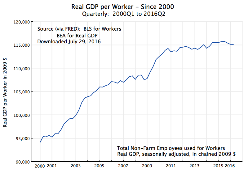
Productivity has increased at a rate of just 0.13% a year since late 2010. This is slow, and a real problem if it continues. I would hasten to add that the period here (5 1/2 years) is still too short to say with any certainty whether this will remain an issue. There have been similar multi-year periods since 1947 when the pace of productivity growth appeared to slow, and then bounced back. Indeed, as seen in the chart above, one would have found a similar pattern had one looked back in early 2009, with a slow pace of productivity growth observed from about 2005.
There has been a good deal of work done by excellent economists on why productivity growth has been what it was, and what it might be in the future. But there is no consensus. Robert J. Gordon of Northwestern University, considered by many to be the “dean in the field”, takes a pessimistic view on the prospects in his recently published magnum opus “The Rise and Fall of American Growth”. Erik Brynjolfsson and Andrew McAfee of MIT, in contrast, argue for a more optimistic view in their recent work “The Second Machine Age” (although “optimistic” might not be the right word because of their concern for the implication of this for jobs). They see productivity growth progressing rapidly, if not accelerating.
But such explanations are focused on possible productivity growth as dictated by what is possible technologically. A separate factor, I would argue, is whether investment in fact takes place that makes use of the technology that is available. And this may well be a dominant consideration when examining the change in productivity over the short and medium terms. A technology is irrelevant if it is not incorporated into the actual production process. And it is only incorporated into the production process via investment.
To understand productivity growth, and why it has fallen in recent decades and perhaps especially so in recent years, one must therefore also look at the investment taking place, and why it is what it is. The rest of this blog post will do that.
B. The Slowdown in the Pace of Investment
The first point to note is that net investment (i.e. after depreciation) has been falling in recent decades when expressed as a share of GDP, with this true for both private and public investment:
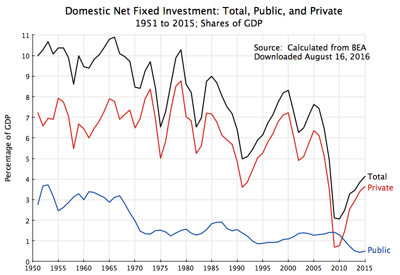
Total net investment has been on a clear downward trend since the mid-1960s. Private net investment has been volatile, falling sharply with the onset of an economic downturn and then recovering. But since the late 1970s its trend has also clearly been downward. Net private investment has been less than 3 1/2% of GDP in recent years, or less than half what it averaged between 1951 and 1980 (of over 7% of GDP). And net public investment, while less volatile, has plummeted over time. It averaged 3.1% of GDP between 1951 and 1968, but is only 0.5% of GDP now (as of 2015), or less than one-sixth of what it was before.
With falling net investment, the rates of growth of public and private capital stocks (fixed assets) have fallen (where 2014 is the most recent year for which the BEA has released such data):

Indeed, expressed in per capita terms, the stock of public capital is now falling. The decrepit state of our highways, bridges, and other public infrastructure should not be a surprise. And the stock of private capital fell each year between 2009 and 2011, with some recovery since but still at almost record low growth.
Even setting aside the recent low (or even negative) figures, the trend in the pace of growth for both public and private capital has declined since the mid-1960s. Why might this be?
C. Why Has Investment Slowed?
The answer is simple and clear for pubic capital. Conservative politicians, in both the US Congress and in many states, have forced cuts in public investment over the years to the current low levels. For whatever reasons, whether ideological or something else, conservative politicians have insisted on cutting or even blocking much of what the United States used to invest in publicly.
Yet public, like private, investment is important to productivity. It is not only commuters trying to get to work who spend time in traffic jams from inadequate roads, and hence face work days of not 8 1/2 hours, but rather 10 or 11 or even 12 hours (with consequent adverse impacts on their productivity). It affects also truck drivers and repairmen, who can accomplish less on their jobs due to time spent in jams. Or, as a consequence of inadequate public investment in computer technology, a greater number of public sector workers are required than otherwise, in jobs ranging from issuing driver’s licenses to enrolling people in Medicare. Inadequate public investment can hold back economic productivity in many ways.
The reasons behind the fall in private investment are less obvious, but more interesting. An obvious possible cause to check is whether private profitability has fallen. If it has, then a reduction in private investment relative to output would not be a surprise. But this has in fact not been the case:

The nominal rate of return on private investment has not only been high, but also surprisingly steady over the years. Profits are defined here as the net operating surplus of all private entities, and is taken from the national account figures of the BEA. They are then taken as a ratio to the stock of private produced assets (fixed assets plus inventories) as of the beginning of the year. This rate of return has varied only between 8 and 13% over the period since at least 1951, and over the last several years has been around 11%.
Many might be surprised by both this high level of profitability and its lack of volatility. I was. But it should be noted that the measure of profitability here, net operating surplus, is a broad measure of all the returns to capital. It includes not only corporate profitability, but also profits of unincorporated businesses, payments of interest (on borrowed capital), and payments of rents (as on buildings). That is, this is the return on all forms of private productive capital in the economy.
The real rates of return have been more volatile, and were especially low between 1974 and 1983, when inflation was high. They are measured here by adjusting the nominal returns for inflation, using the GDP deflator as the measure for inflation. But this real rate of return was a good 9.6% in 2015. That is high for a real rate of return. It was higher than that only for one year late in the Clinton administration, and for several years between the early 1950s and the mid-1960s. But it was never higher than 11%. The current real rate of return on private capital is far from low.
Why then has private investment slowed, in relation to output, if profitability is as high now as it has ever been since the 1950s? One could conceive of several possible reasons. They include:
a) Along the lines of what Robert Gordon has argued, perhaps the underlying pace of technological progress has slowed, and thus there is less of an incentive to undertake new investments (since the returns to replacing old capital with new capital will be less). The rate of growth of capital then slows, and this keeps up profitability (as the capital becomes more scarce relative to output) even as the attractiveness of new investment diminishes.
b) Conservatives might argue that the reduced pace of investment could be due to increased governmental regulations, which makes investment more difficult and raises its cost. This might be difficult to reconcile with the rate of return on capital nonetheless remaining high, but in principle could be if one argues that the slower pace of new investment keeps up profitability as capital then becomes more scarce relative to output. But note that this argument would require that the increased burden of regulation began during the Reagan years in the early 1980s (when the share of private investment in GDP first started to slow – see the chart above), and built up steadily since then through both Republican and Democratic administrations. It would not be something that started only recently under Obama.
c) One could also argue that the reduced investment might be a consequence of “Baumol’s Cost Disease”. This was discussed in earlier posts on this blog, both for overall government spending and for government investment in infrastructure specifically. As discussed in those posts, Baumol’s Cost Disease explains why activities where productivity growth may be relatively more difficult to achieve than in other activities, will see their relative costs increase over time. Construction is an example, where productivity growth has been historically more difficult to achieve than has been the case in manufacturing. Thus the cost of investing, both public and private, relative to the cost of other items will increase over time. This can then also be a possible explanation of slowing new investment, with that slower investment then keeping profitability up due to increasing scarcity of capital.
One problem with each of the possible explanations described above is that they all depend on capital investments becoming less attractive than before, either due to higher costs or due to reduced prospective return. If such factors were indeed critical, one would need to take into account also the effect of taxes on investment returns. And such taxes have been cut sharply over this same period. As discussed in an earlier blog post, taxes on corporate profits, for example, are taxed now at an effective rate of less than 20%, based on what is actually paid after all the legal deductions and credits are included. And this tax rate has fallen steadily over time. The current 20% rate is less than half the effective rate that applied in the 1950s and 1960s, when the effective rate averaged almost 45%. And the tax rate on long-term capital gains, as would apply to returns on capital to individuals, fell from a peak of just below 40% in the mid-1970s to just 15% following the Bush II tax cuts and to 20% since 2013.
Such sharp cuts in taxes on profits implies that the after-tax rate of return on assets has risen sharply (the before-tax rate of return, shown on the chart above, has been flat). Yet despite this, private investment has fallen steadily since the early 1980s as a share of GDP.
Such explanations for the reason behind the fall in private investment since the early 1980s are therefore questionable. However, the purpose of this blog post is not to debate this. Economists are good at coming up with models, possibly convoluted, which can explain things ex post. Several could apply here.
Rather, I would suggest that there might be an alternative explanation for why private investment has been declining. While consistent with basic economics, I have not seen it before. This explanation focuses on the stagnant real wages seen since the early 1980s, and the impact this would have on whether or not to invest.
D. The Impact of Low Real Wages
Real wages have stagnated in the US since the early 1980s, as has been discussed in earlier posts on this blog (see in particular this post). The chart below, updated to the most recent figures available, compares the real median wage since 1979 (the earliest year available for this data series) to real GDP per worker employed:

Real median wages have been flat overall: Just 3% higher in 2016 than what they were 37 years before. But real GDP per worker is almost 60% higher over this same period. This has critically important implications for both private investment and for productivity growth. To sum up in one line the discussion that will follow below, there is less and less reason to invest in new, productivity enhancing, capital, if labor is available at a stagnant real wage that has changed little in 37 years.
Traditional economics, as commonly taught, would find it difficult to explain the observed stagnation in real wages while productivity has risen (even if at a slower pace than before). A core result taught in microeconomics is that in “perfectly competitive” markets, labor will be paid the value of its marginal product. One would not then see a divergence such as that seen in this chart between growth in productivity and a lack of growth in the real wage.
(The more careful observers among the readers of this post might note that the productivity curve shown here is for average productivity, and not the marginal productivity of an extra worker. This is true. Marginal productivity for the economy as a whole cannot be easily observed, nor indeed even be well defined. However, one should note that the average productivity curve, as shown here, is rising over time. This can only happen if marginal productivity on new investments are above average productivity at any point in time. For other reasons, the real average wage would not rise permanently above average productivity (there would be an “adding-up” problem otherwise), but the theory would still predict a rise in the real wage with the increase in observed productivity.)
There are, however, clear reasons why workers might not be paid the value of their marginal product in the real world. As noted, the theory applies in markets that are assumed to be perfectly competitive, and there are many reasons why this is not the case in the world we live in. Perfect competition assumes that both parties to the transaction (the workers and employers) have complete information on not only the opportunities available in the market and on the abilities of the individual worker, but also that there are no costs to switching to an alternative worker or employer. If there is a job on the other side of the country that would pay the individual worker a bit more, then the theory assumes the worker will switch to it. But there are, of course, significant costs to moving to the other side of the country. Furthermore, there will be uncertainty on what the abilities of any individual worker will be, so employers will normally seek to keep the workers they already have to fill their needs (as they know what these workers can do), than take a risk on a largely unknown new worker who might be willing to work for a lower wage.
For these and other reasons, labor markets are not perfectly competitive, and one should not then be surprised to find workers are not being paid the value of their marginal product. But there is also an important factor coming from the macroeconomy. Microeconomics assumes that all resources, including labor resources, are being fully employed. But unemployment exists and is often substantial. Additional workers can then be hired at the current wage, without a need for the firm to raise that wage. And that will hold whether or not the productivity of those workers has risen.
In such an environment, when unemployment is substantial one should not be surprised to find a divergence between growth in productivity and growth in the real wage. And while there have of course been sharp fluctuations arising from the business cycle in the rate of unemployment from year to year, the simple average in the rate since 1979 has been 6.4%. This is well in excess of what is normally considered the full employment rate of unemployment (of 5% or less). Macro policy (both fiscal and monetary) has not done a very good job in most of the years since 1979 in ensuring there is sufficient demand in the aggregate in the economy to allow all workers who want to be employed in fact to be employed.
In such an environment, of workers being available for hire at a stagnant real wage which over time diverges more and more from their productivity, consider the investment decision a private firm faces. Suppose they see a market opportunity and can sell more. To produce more, they have two options. They can hire more labor to work with their existing plant and equipment to produce more, or they can invest in new plant and equipment. If they choose the latter, they can produce more with fewer workers than they would otherwise need at the new level of production. There will be more output per unit of labor input, or put another way, productivity will rise if the latter option is chosen.
But in an economy where labor is available at a flat real wage that has not changed in decades, the best choice will often simply be to hire more labor. The labor is cheap. New investment has a cost, and if the cost of the alternative (hire more labor) is low enough, then it is more profitable for the firm simply to hire more labor. Productivity in such a case will then not go up, and may indeed even go down. But this could be the economically wise choice, if labor is cheap enough.
Viewed in this way, one can see that the interpretation of many conservatives on the relationship between productivity growth and the real wage has it backwards. Real wages have not been stagnant because productivity growth has been slow. Labor productivity since 1979 has grown by a cumulative 60%, while real median wages have been basically flat.
Rather, the causation may well be going the other way. Stagnant and low real wages have led to less and less of an incentive for private firms to invest. And such a cut-back is precisely what we saw in the chart above on private (as well as public) investment as a share of GDP. With less investment, the pace of productivity growth has then slowed.
As a reflection of this confusion, conservatives have denounced any effort to raise wages, asserting that if this is done, jobs will be lost as firms choose instead to invest and automate. They assert that raising the minimum wage, which is currently lower in real terms than what it was when Harry Truman was president, would lead to minimum wage workers losing their jobs. As a former CEO of McDonalds put it in a widely cited news report from last May, a $15 minimum wage would lead to “a job loss like you can’t believe.” Fast food outlets like McDonalds would then find it better to invest in robotic arms to bag the french fries, he said, rather than hire workers to do this.
This is true. The confusion comes from the widespread presumption that this is necessarily bad. Outlets like McDonalds would then require fewer workers, but they would still need workers (including to operate the robotic arms), and those workers would be more productive. They could be paid more, and would be if the minimum wage is raised.
The error in the argument comes from the presumption that the workers being employed at the current minimum wage of $7.25 an hour do not and can not possess the skills needed to be employed in some other job. There is no reason to believe this to be the case. There was no problem with ensuring workers could be fully employed at a minimum wage which in real terms was higher in 1950, when Harry Truman was president, than what it is now. And average worker productivity is 2.4 times higher now than what it was then.
Ensuring full employment in the economy as a whole is not a responsibility of private business. Rather, it is a government responsibility. Fiscal and monetary policy need to be managed so that labor markets are tight enough to ensure all workers who want a job can get a job, while not so tight at to lead to inflation.
Following the economic collapse at the end of the Bush administration in 2008, monetary policy did all it could to try to ensure sufficient aggregate demand in the economy (interest rates were held at or close to zero). But monetary policy alone will not be enough when the economy collapsed as far as it did in 2008. It needs to be complemented by supportive fiscal policy. While there was the initial stimulus package of Obama which was critical to stabilizing the economy, it did not go far enough and was allowed to run out. And government spending from 2010 was then cut, acting as a drag which kept the pace of recovery slow. The economy has only in the past year returned to close to full employment. It is not a coincidence that real wages are finally starting to rise (as seen in the chart above).
E. Conclusion
Productivity growth is key in any economy. Over the long run, living standards can only improve if productivity does. Hence there is reason to be concerned with the slower pace of productivity growth seen since the early 1980s, and especially in recent years.
Investment, both public and private, is what leads to productivity growth, but the pace of investment has slowed since the levels seen in the 1950s and 60s. The cause of the decline in public investment is clear: Conservative politicians have slowed or even blocked public investment. The result is obvious in our public infrastructure: It is overused, under-maintained, and often an embarrassment.
The cause of the slowdown in private investment is less obvious, but equally important. First, one cannot blame a decline in private investment on a fall in profitability: Profitability is higher now than it has been in all but one year since the mid-1960s.
Rather, one needs to recognize that the incentive to invest in productivity enhancing tools will not be there (or not there to the same extent) if labor can be hired at a wage that has stagnated for decades, and which over time became lower and lower relative to existing productivity. It then makes more sense for firms to hire more workers with their existing stock of capital and other equipment, rather than invest in new, productivity enhancing, capital. And this is what we have observed: Workers are being hired, but productivity is not growing.
An argument is often made that if firms did indeed invest in capital and equipment that would raise productivity, that workers would then lose their jobs. This is actually true by definition: If productivity is higher, then the firm needs fewer workers per unit of output than they would otherwise. But whether more workers would be employed in the economy as a whole does not depend on the actions of any individual firm, but rather on whether fiscal and monetary policy is managed to ensure full employment.
That is, it is the investment decisions of private firms which determine whether productivity will grow or not. It is the macro management decisions of government which determine whether workers will be fully employed or not.
To put this bluntly, and in simplistic “bumper sticker” type terms, one could say that private businesses are not job creators, but rather job destroyers. And that is fine. Higher productivity means that a firm needs fewer workers to produce what they make than would otherwise have been needed, and this is important for ensuring efficiency. As a necessary complement to this, however, it is the actions of government, through its fiscal and monetary policies, which “creates” jobs by managing aggregate demand to ensure all workers who want to be employed, are employed.



 An Economic Sense
You must be logged in to post a comment.