Andrew Yang’s Proposed $1,000 per Month Grant: Issues Raised in the Democratic Debate

A.  Introduction

This is the second in a series of posts on this blog addressing issues that have come up during the campaign of the candidates for the Democratic nomination for president, and which specifically came up in the October 15 Democratic debate.  As flagged in the previous blog post, one can find a transcript of the debate at the Washington Post website, and a video of the debate at the CNN website.

This post will address Andrew Yang’s proposal of a $1,000 per month grant for every adult American (which I will mostly refer to here as a $12,000 grant per year).  This policy is called a universal basic income (or UBI), and has been explored in a few other countries as well.  It has received increased attention in recent years, in part due to the sharp growth in income inequality in the US of recent decades, that began around 1980.  If properly designed, such a $12,000 grant per adult per year could mark a substantial redistribution of income.  But the degree of redistribution depends directly on how the funding would be raised.  As we will discuss below, Yang’s specific proposals for that are problematic.  There are also other issues with such a program which, even if well designed, calls into question whether it would be the best approach to addressing inequality.  All this will be discussed below.

First, however, it is useful to address two misconceptions that appear to be widespread.  One is that many appear to believe that the $12,000 per adult per year would not need to come from somewhere.  That is, everyone would receive it, but no one would have to provide the funds to pay for it.  That is not possible.  The economy produces so much, whatever is produced accrues as incomes to someone, and if one is to transfer some amount ($12,000 here) to each adult then the amounts so transferred will need to come from somewhere.  That is, this is a redistribution.  There is nothing wrong with a redistribution, if well designed, but it is not a magical creation of something out of nothing.

The other misconception, and asserted by Yang as the primary rationale for such a $12,000 per year grant, is that a “Fourth Industrial Revolution” is now underway which will lead to widespread structural unemployment due to automation.  This issue was addressed in the previous post on this blog, where I noted that the forecast job losses due to automation in the coming years are not out of line with what has been the norm in the US for at least the last 150 years.  There has always been job disruption and turnover, and while assistance should certainly be provided to workers whose jobs will be affected, what is expected in the years going forward is similar to what we have had in the past.

It is also a good thing that workers should not be expected to rely on a $12,000 per year grant to make up for a lost job.  Median earnings of a full-time worker was an estimated $50,653 in 2018, according to the Census Bureau.  A grant of $12,000 would not go far in making up for this.

So the issue is one of redistribution, and to be fair to Yang, I should note that he posts on his campaign website a fair amount of detail on how the program would be paid for.  I make use of that information below.  But the numbers do not really add up, and for a candidate who champions math (something I admire), this is disappointing.

B.  Yang’s Proposal of a $1,000 Monthly Grant to All Americans

First of all, the overall cost.  This is easy to calculate, although not much discussed.  The $12,000 per year grant would go to every adult American, who Yang defines as all those over the age of 18.  There were very close to 250 million Americans over the age of 18 in 2018, so at $12,000 per adult the cost would be $3.0 trillion.

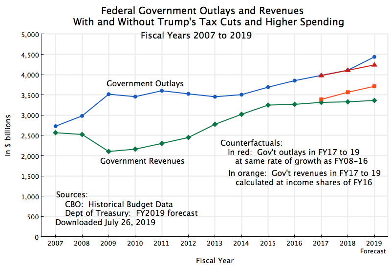
This is far from a small amount.  With GDP of approximately $20 trillion in 2018 ($20.58 trillion to be more precise), such a program would come to 15% of GDP.  That is huge.  Total taxes and revenues received by the federal government (including all income taxes, all taxes for Social Security and Medicare, and everything else) only came to $3.3 trillion in FY2018.  This is only 10% more than the $3.0 trillion that would have been required for Yang’s $12,000 per adult grants.  Or put another way, taxes and other government revenues would need almost to be doubled (raised by 91%) to cover the cost of the program.  As another comparison, the cost of the tax cuts that Trump and the Republican leadership rushed through Congress in December 2017 was forecast to be an estimated $150 billion per year.  That was a big revenue loss.  But the Yang proposal would cost 20 times as much.

With such amounts to be raised, Yang proposes on his campaign website a number of taxes and other measures to fund the program.  One is a value-added tax (VAT), and from his very brief statements during the debates but also in interviews with the media, one gets the impression that all of the program would be funded by a value-added tax.  But that is not the case.  He in fact says on his campaign website that the VAT, at the rate and coverage he would set, would raise only about $800 billion.  This would come only to a bit over a quarter (27%) of the $3.0 trillion needed.  There is a need for much more besides, and to his credit, he presents plans for most (although not all) of this.

So what does he propose specifically?:

a) A New Value-Added Tax:

First, and as much noted, he is proposing that the US institute a VAT at a rate of 10%.  He estimates it would raise approximately $800 billion a year, and for the parameters for the tax that he sets, that is a reasonable estimate.  A VAT is common in most of the rest of the world as it is a tax that is relatively easy to collect, with internal checks that make underreporting difficult.  It is in essence a tax on consumption, similar to a sales tax but levied only on the added value at each stage in the production chain.  Yang notes that a 10% rate would be approximately half of the rates found in Europe (which is more or less correct – the rates in Europe in fact vary by country and are between 17 and 27% in the EU countries, but the rates for most of the larger economies are in the 19 to 22% range).

A VAT is a tax on what households consume, and for that reason a regressive tax.  The poor and middle classes who have to spend all or most of their current incomes to meet their family needs will pay a higher share of their incomes under such a tax than higher-income households will.  For this reason, VAT systems as implemented will often exempt (or tax at a reduced rate) certain basic goods such as foodstuffs and other necessities, as such goods account for a particularly high share of the expenditures of the poor and middle classes.  Yang is proposing this as well.  But even with such exemptions (or lower VAT rates), a VAT tax is still normally regressive, just less so.

Furthermore, households will in the end be paying the tax, as prices will rise to reflect the new tax.  Yang asserts that some of the cost of the VAT will be shifted to businesses, who would not be able, he says, to pass along the full cost of the tax.  But this is not correct.  In the case where the VAT applies equally to all goods, the full 10% will be passed along as all goods are affected equally by the now higher cost, and relative prices will not change.  To the extent that certain goods (such as foodstuffs and other necessities) are exempted, there could be some shift in demand to such goods, but the degree will depend on the extent to which they are substitutable for the goods which are taxed.  If they really are necessities, such substitution is likely to be limited.

A VAT as Yang proposes thus would raise a substantial amount of revenues, and the $800 billion figure is a reasonable estimate.  This total would be on the order of half of all that is now raised by individual income taxes in the US (which was $1,684 billion in FY2018).  But one cannot avoid that such a tax is paid by households, who will face higher prices on what they purchase, and the tax will almost certainly be regressive, impacting the poor and middle classes the most (with the extent dependent on how many and which goods are designated as subject to a reduced VAT rate, or no VAT at all).  But whether regressive or not, everyone will be affected and hence no one will actually see a net increase of $12,000 in purchasing power from the proposed grant  Rather, it will be something less.

b)  A Requirement to Choose Either the $12,000 Grants, or Participation in Existing Government Social Programs

Second, Yang’s proposal would require that households who currently benefit from government social programs, such as for welfare or food stamps, would be required to give up those benefits if they choose to receive the $12,000 per adult per year.  He says this will lead to reduced government spending on such social programs of $500 to $600 billion a year.

There are two big problems with this.  The first is that those programs are not that large.  While it is not fully clear how expansive Yang’s list is of the programs which would then be denied to recipients of the $12,000 grants, even if one included all those included in what the Congressional Budget Office defines as “Income Security” (“unemployment compensation, Supplemental Security Income, the refundable portion of the earned income and child tax credits, the Supplemental Nutrition Assistance Program [food stamps], family support, child nutrition, and foster care”), the total spent in FY2018 was only $285 billion.  You cannot save $500 to $600 billion if you are only spending $285 billion.

Second, such a policy would be regressive in the extreme.  Poor and near-poor households, and only such households, would be forced to choose whether to continue to receive benefits under such existing programs, or receive the $12,000 per adult grant per year.  If they are now receiving $12,000 or more in such programs per adult household member, they would receive no benefit at all from what is being called a “universal” basic income grant.  To the extent they are now receiving less than $12,000 from such programs (per adult), they may gain some benefit, but less than $12,000 worth.  For example, if they are now receiving $10,000 in benefits (per adult) from current programs, their net gain would be just $2,000 (setting aside for the moment the higher prices they would also now need to pay due to the 10% VAT).  Furthermore, only the poor and near-poor who are being supported by such government programs will see such an effective reduction in their $12,000 grants.  The rich and others, who benefit from other government programs, will not see such a cut in the programs or tax subsidies that benefit them.

c)  Savings in Other Government Programs 

Third, Yang argues that with his universal basic income grant, there would be a reduction in government spending of $100 to $200 billion a year from lower expenditures on “health care, incarceration, homelessness services and the like”, as “people would be able to take better care of themselves”.  This is clearly more speculative.  There might be some such benefits, and hopefully would be, but without experience to draw on it is impossible to say how important this would be and whether any such savings would add up to such a figure.  Furthermore, much of those savings, were they to follow, would accrue not to the federal government but rather to state and local governments.  It is at the state and local level where most expenditures on incarceration and homelessness, and to a lesser degree on health care, take place.  They would not accrue to the federal budget.

d)  Increased Tax Revenues From a Larger Economy

Fourth, Yang states that with the $12,000 grants the economy would grow larger – by 12.5% he says (or $2.5 trillion in increased GDP).  He cites a 2017 study produced by scholars at the Roosevelt Institute, a left-leaning non-profit think tank based in New York, which examined the impact on the overall economy, under several scenarios, of precisely such a $12,000 annual grant per adult.

There are, however, several problems:

i)  First, under the specific scenario that is closest to the Yang proposal (where the grants would be funded through a combination of taxes and other actions), the impact on the overall economy forecast in the Roosevelt Institute study would be either zero (when net distribution effects are neutral), or small (up to 2.6%, if funded through a highly progressive set of taxes).

ii)  The reason for this result is that the model used by the Roosevelt Institute researchers assumes that the economy is far from full employment, and that economic output is then entirely driven by aggregate demand.  Thus with a new program such as the $12,000 grants, which is fully paid for by taxes or other measures, there is no impact on aggregate demand (and hence no impact on economic output) when net distributional effects are assumed to be neutral.  If funded in a way that is not distributionally neutral, such as through the use of highly progressive taxes, then there can be some effect, but it would be small.

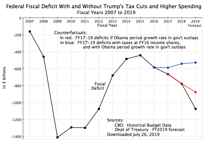
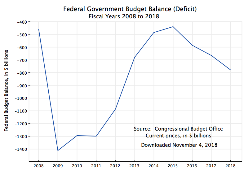
In the Roosevelt Institute model, there is only a substantial expansion of the economy (of about 12.5%) in a scenario where the new $12,000 grants are not funded at all, but rather purely and entirely added to the fiscal deficit and then borrowed.  And with the current fiscal deficit now about 5% of GDP under Trump (unprecedented even at 5% in a time of full employment, other than during World War II), and the $12,000 grants coming to $3.0 trillion or 15% of GDP, this would bring the overall deficit to 20% of GDP!

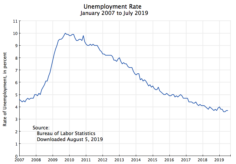
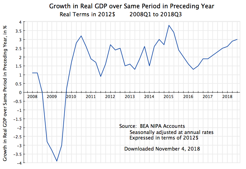
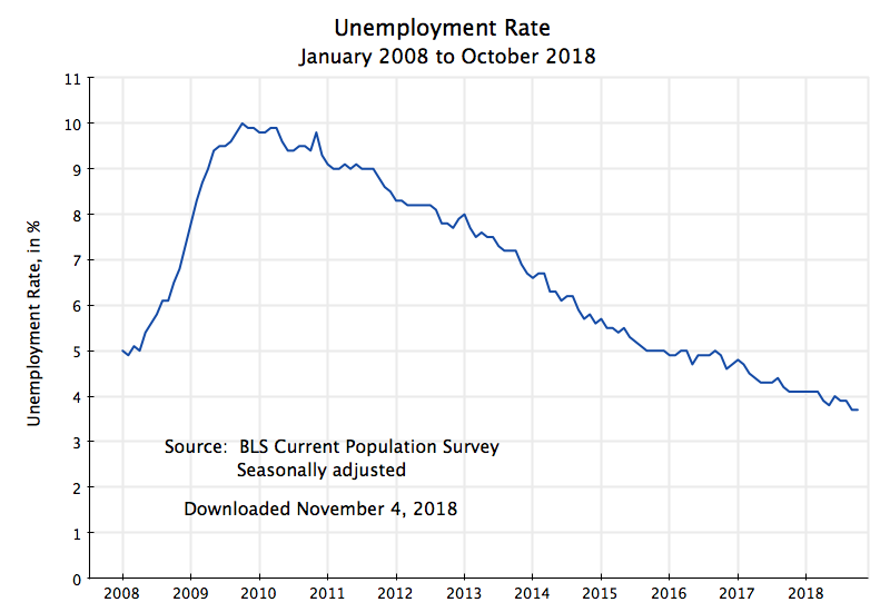
Few economists would accept that such a scenario is anywhere close to plausible.  First of all, the current unemployment rate of 3.5% is at a 50 year low.  The economy is at full employment.  The Roosevelt Institute researchers are asserting that this is fictitious, and that the economy could expand by a substantial amount (12.5% in their scenario) if the government simply spent more and did not raise taxes to cover any share of the cost.  They also assume that a fiscal deficit of 20% of GDP would not have any consequences, such as on interest rates.  Note also an implication of their approach is that the government spending could be on anything, including, for example, the military.  They are using a purely demand-led model.

iii)  Finally, even if one assumes the economy will grow to be 12.5% larger as a result of the grants, even the Roosevelt Institute researchers do not assume it will be instantaneous.  Rather, in their model the economy becomes 12.5% larger only after eight years.  Yang is implicitly assuming it will be immediate.

There are therefore several problems in the interpretation and use of the Roosevelt Institute study.  Their scenario for 12.5% growth is not the one that follows from Yang’s proposals (which is funded, at least to a degree), nor would GDP jump immediately by such an amount.  And the Roosevelt Insitute model of the economy is one that few economists would accept as applicable in the current state of the economy, with its 3.5% unemployment.

But there is also a further problem.  Even assuming GDP rises instantly by 12.5%, leading to an increase in GDP of $2.5 trillion (from a current $20 trillion), Yang then asserts that this higher GDP will generate between $800 and $900 billion in increased federal tax revenue.  That would imply federal taxes of 32 to 36% on the extra output.  But that is implausible.  Total federal tax (and all other) revenues are only 17.5% of GDP.  While in a progressive tax system the marginal tax revenues received on an increase in income will be higher than at the average tax rate, the US system is no longer very progressive.  And the rates are far from what they would need to be twice as high at the margin (32 to 36%) as they are at the average (17.5%).  A more plausible estimate of the increased federal tax revenues from an economy that somehow became 12.5% larger would not be the $800 to $900 billion Yang calculates, but rather about half that.

Might such a universal basic income grant affect the size of the economy through other, more orthodox, channels?  That is certainly possible, although whether it would lead to a higher or to a lower GDP is not clear.  Yang argues that it would lead recipients to manage their health better, to stay in school longer, to less criminality, and to other such social benefits.  Evidence on this is highly limited, but it is in principle conceivable in a program that does properly redistribute income towards those with lower incomes (where, as discussed above, Yang’s specific program has problems).  Over fairly long periods of time (generations really) this could lead to a larger and stronger economy.

But one will also likely see effects working in the other direction.  There might be an increase in spouses (wives usually) who choose to stay home longer to raise their children, or an increase in those who decide to retire earlier than they would have before, or an increase in the average time between jobs by those who lose or quit from one job before they take another, and other such impacts.  Such impacts are not negative in themselves, if they reflect choices voluntarily made and now possible due to a $12,000 annual grant.  But they all would have the effect of reducing GDP, and hence the tax revenues that follow from some level of GDP.

There might therefore be both positive and negative impacts on GDP.  However, the impact of each is likely to be small, will mostly only develop over time, and will to some extent cancel each other out.  What is likely is that there will be little measurable change in GDP in whichever direction.

e)  Other Taxes

Fifth, Yang would institute other taxes to raise further amounts.  He does not specify precisely how much would be raised or what these would be, but provides a possible list and says they would focus on top earners and on pollution.  The list includes a financial transactions tax, ending the favorable tax treatment now given to capital gains and carried interest, removing the ceiling on wages subject to the Social Security tax, and a tax on carbon emissions (with a portion of such a tax allocated to the $12,000 grants).

What would be raised by such new or increased taxes would depend on precisely what the rates would be and what they would cover.  But the total that would be required, under the assumption that the amounts that would be raised (or saved, when existing government programs are cut) from all the measures listed above are as Yang assumes, would then be between $500 and $800 billion (as the revenues or savings from the programs listed above sum to $2.2 to $2.5 trillion).  That is, one might need from these “other taxes” as much as would be raised by the proposed new VAT.

But as noted in the discussion above, the amounts that would be raised by those measures are often likely to be well short of what Yang says will be the case.  One cannot save $500 to $600 billion in government programs for the poor and near-poor if government is spending only $285 billion on such programs, for example.  A more plausible figure for what might be raised by those proposals would be on the order of $1 trillion, mostly from the VAT, and not the $2.2 to $2.5 trillion Yang says will be the case.

C.  An Assessment

Yang provides a fair amount of detail on how he would implement a universal basic income grant of $12,000 per adult per year, and for a political campaign it is an admirable amount of detail.  But there are still, as discussed above, numerous gaps that prevent anything like a complete assessment of the program.  But a number of points are evident.

To start, the figures provided are not always plausible.  The math just does not add up, and for someone who extolls the need for good math (and rightly so), this is disappointing.  One cannot save $500 to $600 billion in programs for the poor and near-poor when only $285 billion is being spent now.  One cannot assume that the economy will jump immediately by 12.5% (which even the Roosevelt Institute model forecasts would only happen in eight years, and under a scenario that is the opposite of that of the Yang program, and in a model that few economists would take as credible in any case).  Even if the economy did jump by so much immediately, one would not see an increase of $800 to $900 billion in federal tax revenues from this but rather more like half that.  And other such issues.

But while the proposal is still not fully spelled out (in particular on which other taxes would be imposed to fill out the program), we can draw a few conclusions.  One is that the one group in society who will clearly not gain from the $12,000 grants is the poor and near-poor, who currently make use of food stamp and other such programs and decide to stay with those programs.  They would then not be eligible for the $12,000 grants.  And keep in mind that $12,000 per adult grants are not much, if you have nothing else.  One would still be below the federal poverty line if single (where the poverty line in 2019 is $12,490) or in a household with two adults and two or more children (where the poverty line, with two children, is $25,750).  On top of this, such households (like all households) will pay higher prices for at least some of what they purchase due to the new VAT.  So such households will clearly lose.

Furthermore, those poor or near-poor households who do decide to switch, thus giving up their eligibility for food stamps and other such programs, will see a net gain that is substantially less than $12,000 per adult.  The extent will depend on how much they receive now from those social programs.  Those who receive the most (up to $12,000 per adult), who are presumably also most likely to be the poorest among them, will lose the most.  This is not a structure that makes sense for a program that is purportedly designed to be of most benefit to the poorest.

For middle and higher-income households the net gain (or loss) from the program will depend on the full set of taxes that would be needed to fund the program.  One cannot say who will gain and who will lose until the structure of that full set of taxes is made clear.  This is of course not surprising, as one needs to keep in mind that this is a program of redistribution:  Funds will be raised (by taxes) that disproportionately affect certain groups, to be distributed then in the $12,000 grants.  Some will gain and some will lose, but overall the balance has to be zero.

One can also conclude that such a program, providing for a universal basic income with grants of $12,000 per adult, will necessarily be hugely expensive.  It would cost $3 trillion a year, which is 15% of GDP.  Funding it would require raising all federal tax and other revenue by 91% (excluding any offset by cuts in government social programs, which are however unlikely to amount to anything close to what Yang assumes).  Raising funds of such magnitude is completely unrealistic.  And yet despite such costs, the grants provided of $12,000 per adult would be poverty level incomes for those who do not have a job or other source of support.

One could address this by scaling back the grant, from $12,000 to something substantially less, but then it becomes less meaningful to an individual.  The fundamental problem is the design as a universal grant, to all adults.  While this might be thought to be politically attractive, any such program then ends up being hugely expensive.

The alternative is to design a program that is specifically targeted to those who need such support.  Rather than attempting to hide the distributional consequences in a program that claims to be universal (but where certain groups will gain and certain groups will lose, once one takes fully into account how it will be funded), make explicit the redistribution that is being sought.  With this clear, one can then design a focussed program that addresses that redistribution aim.

Finally, one should recognize that there are other policies as well that might achieve those aims that may not require explicit government-intermediated redistribution.  For example, Senator Cory Booker in the October 15 debate noted that a $15 per hour minimum wage would provide more to those now at the minimum wage than a $12,000 annual grant.  This remark was not much noted, but what Senator Booker said was true.  The federal minimum wage is currently $7.25 per hour.  This is low – indeed, it is less (in real terms) than what it was when Harry Truman was president.  If the minimum wage were raised to $15 per hour, a worker now at the $7.25 rate would see an increase in income of $15.00 – $7.25 = $7.75 per hour, and over a year of 40 hour weeks would see an increase in income of $7.75 x 40 x 52 = $16,120.00.  This is well more than a $12,000 annual grant would provide.

Republican politicians have argued that raising the minimum wage by such a magnitude will lead to widespread unemployment.  But there is no evidence that changes in the minimum wage that we have periodically had in the past (whether federal or state level minimum wages) have had such an adverse effect.  There is of course certainly some limit to how much it can be raised, but one should recognize that the minimum wage would now be over $24 per hour if it had been allowed to grow at the same pace as labor productivity since the late 1960s.

Income inequality is a real problem in the US, and needs to be addressed.  But there are problems with Yang’s specific version of a universal basic income.  While one may be able to fix at least some of those problems and come up with something more reasonable, it would still be massively disruptive given the amounts to be raised.  And politically impossible.  A focus on more targeted programs, as well as on issues such as the minimum wage, are likely to prove far more productive.

The Growing Fiscal Deficit, the Keynesian Stimulus Policies of Trump, and the FY20/21 Budget Agreement

A.  The Growing Fiscal Deficit Under Trump

Donald Trump, when campaigning for office, promised that he would “quickly” drive down the fiscal deficit to zero.  Few serious analysts believed that he would get it all the way to zero during his term in office, but many assumed that he would at least try to reduce the deficit by some amount.  And this clearly should have been possible, had he sought to do so, when Republicans were in full control of both the House and the Senate, as well as the presidency.

That has not happened.  The deficit has grown markedly, despite the economy being at full employment, and is expected to top $1 trillion this year, reaching over 5% of GDP.  This is unprecedented in peacetime.  Never before in US history, other than during World War II, has the federal deficit hit 5% of GDP with the economy at full employment.  Indeed, the fiscal deficit has never even reached 4% of GDP at a time of full employment (other than, again, World War II).

The chart at the top of this post shows what has happened.  The deficit is the difference between what the government spends (shown as the line in blue) and the revenues it receives (the line in green).  The deficit grew markedly following the financial and economic collapse in the last year of the Bush administration.  A combination of higher government spending and lower taxes (lower both because the economy was depressed but also from legislated tax cuts) were then necessary to stabilize the economy.  As the economy recovered the fiscal deficit then narrowed.  But it is now widening again, and as noted above, is expected to top $1 trillion dollars in FY2019 (which ends on September 30).

More precisely, the US Treasury publishes monthly a detailed report on what the federal government received in revenues and what was spent in outlays for that month and for up to that point in the fiscal year.  See here for the June report, and here for previous monthly reports.  It includes a forecast of what will be received and spent for the fiscal year as a whole, and hence what the deficit will be, based on the budget report released each spring, usually in March.  For FY2019, the forecast was of a deficit of $1.092 trillion.  But these are forecasts, and comparing the forecasts made to the actuals realized over the last three fiscal years (FY2016 to18), government outlays were on average overestimated by 2.0% and government revenues by 2.2%.  These are similar, and scaling the forecasts of government outlays and government revenues down by these ratios, the deficit would end up at $1.075 trillion.  I used these scaled figures in the chart above.

The widening in the deficit in recent years is evident.  The interesting question is why.  For this one needs counterfactuals, of what the figures would have been if some alternative decisions had been made.

For government revenues (taxes of various kinds), the curve in orange show what they would have been had taxes remained at the same shares of the relevant income (depending on the tax) as they were in FY2016.  Specifically, individual income taxes were kept at a constant share of personal income (as defined and estimated in the National Income and Product Accounts, or NIPA accounts, assembled by the Bureau of Economic Analysis, or BEA, of the US Department of Commerce); corporate profit taxes were kept at a constant share of corporate profits (as estimated in the NIPA accounts); payroll taxes (primarily Social Security taxes) were kept at a constant share of compensation of employees (again from the NIPA accounts); and all other taxes were kept at a constant share of GDP.  The NIPA accounts (often referred to as the GDP accounts) are available through the second quarter of CY2019, and hence are not yet available for the final quarter of FY2019 (which ends September 30, and hence includes the third quarter of CY2019).  For this, I extrapolated the final quarter’s figures based on what growth had been over the preceding four quarters.

Note also that the base year here (FY2016) already shows a flattening in tax revenues.  If I had used the tax shares of FY2015 as a base for the comparison, the tax losses in the years since then would have been even greater.  Various factors account for the flattening of tax revenues in FY2016, including (according to an analysis by the Congressional Budget Office) passage by Congress of Public Law 114-113 in December 2015, that allowed for a more rapid acceleration of depreciation allowances for investment by businesses.  This had the effect of reducing corporate profit taxes substantially in FY2016.

Had taxes remained at the shares of the relevant income as they were in FY2016, tax revenues would have grown, following the path of the orange curve.  Instead, they were flat in nominal dollar amount (the green curve), indicating they were falling in real terms as well as a share of income.  The largest loss in revenues stemmed from the major tax cut pushed through Congress in December 2017, which took effect on January 1, 2018.  Hence it applied over three of the four quarters in FY2018, and for all of FY2019.

An increase in government spending is also now leading, in FY2019, to a widening of the deficit.  Again, one needs to define a counterfactual for the comparison.  For this I assumed that government spending during Trump’s term in office so far would have grown at the same rate as it had during Obama’s eight years in office (the rate of increase from FY2008 to 16).  That rate of increase during Obama’s two terms was 3.2% a year (in nominal terms), and was substantially less than during Bush’s two terms (which was a 6.6% rate of growth per year).

The rate of growth in government spending in the first two years of Trump’s term (FY2017 and 2018) then almost exactly matched the rate of growth under Obama.  But this has now changed sharply in FY19, with government spending expected to jump by 8.0% in just one year.

The fiscal deficit is then the difference, as noted above, between the two curves for spending and revenues.  Its change over time may be clearer in a chart of just the deficit itself:

The curve in black shows what the deficit has been, and what is expected for FY2019.  The deficit narrowed to $442 billion in FY2015, and then started to widen.  Primarily due to flat tax revenues in FY2016 (spending was following the path it had been following before, after several years of suppression), the deficit grew in FY2016.  And it then continued to grow until at least through FY2019.  The curve in red shows what the deficit would have been had government spending continued to grow under Trump at the pace it had under Obama.  This would have made essentially no difference in FY2017 and FY2018, but would have reduced the deficit in FY2019 from the expected $1,075 billion to $877 billion instead.  Not a small deficit by any means, but not as high.

But more important has been the contribution to the higher deficit from tax cuts.  The combined effect is shown in the curve in blue in the chart.  The deficit would have stabilized and in fact reduced by a bit.  For FY2019, the deficit would have been $528 billion, or a reasonable 2.5% of GDP.  Instead, at an expected $1,075 billion, it will be over twice as high.  And it is a consequence of Trump’s policies.

B.  Have the Tax Cuts Led to Higher Growth?

The Trump administration claimed that the tax cuts (and specifically the major cuts passed in December 2017) would lead to such a more rapid pace of GDP growth that they would “pay for themselves”.  This clearly has not happened – tax revenues have fallen in real terms (they were flat in nominal terms).  But a less extreme argument was that the tax cuts, and in particular the extremely sharp cut in corporate profit taxes, would lead to a spurt of new corporate investment in equipment, which would raise productivity and hence GDP.  See, for example, the analysis issued by the White House Council of Economic Advisors in October 2017.

But this has not happened either.  Growth in private investment in equipment has in fact declined since the first quarter of 2018 (when the law went into effect):

The curve in blue shows the quarter to quarter changes (at an annual rate), while the curve in red smooths this out by showing the change over the same quarter of a year earlier.  There is a good deal of volatility in the quarter to quarter figures, while the year on year changes show perhaps some trends that last perhaps two years or so, but with no evidence that the tax cut led to a spurt in such investment.  The growth has in fact slowed.

Such investment is in fact driven largely by more fundamental factors, not by taxes.  There was a sharp fall in 2008 as a result of the broad economic and financial collapse at the end of the Bush administration, it then bounced back in 2009/10, and has fluctuated since driven by various industry factors.  For example, oil prices as well as agricultural prices both fell sharply in 2015, and the NIPA accounts indicate that equipment investment in just these two sectors reduced private investment in equipment by more than 2% points from what the total would have been in 2015.  This continued into 2016, with a reduction of a further 1.3% points.  What matters are the fundamentals.  Taxes are secondary, at best.

What about GDP itself?:

Here again there is quarter to quarter volatility, but no evidence that the tax cuts have spurred GDP growth.  Over the past three years, real GDP growth on a quarter to quarter basis peaked in the fourth quarter of 2017, before the tax cuts went into effect, and has declined modestly since then.  And that peak in the fourth quarter of 2017 was not anything special:  GDP grew at a substantially faster pace in the second and third quarters of 2014, and the year on year rate in early 2015 was higher than anything reached in 2017-19.  Rather, what we see in real GDP growth since late 2009 is significant quarter to quarter volatility, but around an average pace of about 2.3% a year.  There is no evidence that the late 2017 tax cut has raised this.

The argument that tax cuts will spur private investment, and hence productivity and hence GDP, is a supply-side argument.  There is no evidence in the numbers to support this.  But there may also be a demand-side argument, which is basically Keynesian.  The argument would be that tax cuts lead to higher (after-tax) incomes, and that these higher incomes led to higher consumption expenditures by households.  There might be some basis to this, to the extent that a portion of the tax cuts went to low and middle-income households who will spend more upon receiving it.  But since the tax cut law passed in December 2017 went primarily to the rich, whose consumption is not constrained by their current income flows (they save the excess), the impact of the tax cuts on household consumption would be weak.  It still, however, might be something.

But this still did not lead to a more rapid pace of GDP growth, as we saw above.  Why?  One needs to recognize that GDP is a measure of production in the domestic economy (GDP is Gross Domestic Product), and not of demand.  GDP is commonly measured by adding up the components of demand, with any increase or decrease in the stock of inventories then added (or subtracted, if negative) to tell us what production must have been.  But this is being done because the data is better (and more quickly available) for the components of GDP demand.  One must not forget that GDP is still an estimate of production, and not of total domestic demand.

And what the economy can produce when at full employment is constrained by whatever capacity was at that point in time.  The rate of unemployment has fallen steadily since hitting its peak in 2009 during the downturn:

Aside from the “squiggles” in these monthly figures (the data are obtained from household surveys, and will be noisy), unemployment fell at a remarkably steady pace since 2009.  One can also not discern any sharp change in that pace before and after January 2017, when Trump took office.  But the rate of unemployment is now leveling off, as it must, since there will always be some degree of frictional unemployment when an economy is at “full employment”.

With the economy at full employment, growth will now be constrained by the pace of growth of the labor force (about 0.5% a year) plus the growth in productivity of the average labor force member (which analysts, such as at the Congressional Budget Office, put at about 1.5% a year in the long term, and a bit less over the next decade).  That is, growth in GDP capacity will be 2% a year, or less, on average.

In such situations, Keynesian demand expansion will not raise the growth in GDP beyond that 2% rate.  There will of course be quarter to quarter fluctuations (GDP growth estimates are volatile), but on average over time, one should not expect growth in excess of this.

But growth can be less.  In a downturn, such as that suffered in 2008/09, GDP growth can drop well below capacity.  Unemployment soars, and Keynesian demand stimulus is needed to stabilize the economy and return it to a growth path.  Tax cuts (when focused on low and middle income households) can be stimulative.  But especially stimulative in such circumstances is direct government spending, as such spending leads directly to people being hired and put to work.

Thus the expansion in government spending in 2008/09 (see the chart at the top of this post) was exactly what was needed in those circumstances.  The mistake then was to hold government spending flat in nominal terms (and hence falling in real terms) between 2009 and 2014, even though unemployment, while falling, was still relatively high.  That cut-back in government spending was unprecedented in a period of recovery from a downturn (over at least the past half-century in the US).  And an earlier post on this blog estimated that had government spending been allowed to increase at the same pace as it had under Reagan following the 1982 downturn, the US economy would have fully recovered by 2012.

But the economy is now at full employment.  In these circumstances, extra demand stimulus will not increase production (as production is limited by capacity), but will rather spill over into a drawdown in inventories (in the short term, but there is only so much in inventories that one can draw down) or an increase in the trade deficit (more imports to satisfy the domestic demand, or exports diverted to meet the domestic demand).  One saw this in the initial estimates for the GDP figures for the second quarter of 2019.  GDP is estimated to have grown at a 2.1% rate.  But the domestic final demand components grew at a pace that, by themselves, would have accounted for a 3.6% point increase in GDP.  The difference was accounted for by a drawdown in inventories (accounting for 0.7% points of GDP) and an increase in the trade deficit (accounting for a further reduction of 0.8% points of GDP).  But these are just one quarter of figures, they are volatile, and it remains to be seen whether this will continue.

It is conceivable that domestic demand might fall back to grow in line with capacity.  But this then brings up what should be considered the second arm of Trump’s Keynesian stimulus program.  While tax cuts led to growing deficits in FY2017 and 18, we are now seeing in FY2019, in addition to the tax cuts, an extraordinary growth in government spending.  Based on US Treasury forecasts for FY2019 (as adjusted above), federal government spending this fiscal year is expected to grow by 8.0%.  This will add to domestic demand growth.  And there has not been such growth in government spending during a time of full employment since George H. W. Bush was president.

C.  The Impact of the Bipartisan Budget Act of 2019

Just before leaving for its summer recess, the House and the Senate in late July both passed an important bill setting the budget parameters for fiscal years 2020 and 2021.  Trump signed it into law on August 2.  It was needed as, under the budget sequester process forced on Obama in 2011, there would have otherwise been sharp cutbacks in the discretionary budgets for what government is allowed to spend (other than for programs such as Social Security or Medicare, where spending follows the terms of the programs as established, or for what is spent on interest on the public debt).  The sequesters would have set sharp cuts in government spending in fiscal years 2020 and 2021, and if allowed, such sudden cuts could have pushed the US economy into a recession.

The impact is clear on a chart:

The figures are derived from the Congressional Budget Office analysis of the impact on government spending from the lifting of the caps.  Without the change in the spending caps, discretionary spending would have been sharply reduced.  At the new caps, spending will increase at a similar pace as it had before.

Note the sharp contrast with the cut-backs in discretionary budget outlays from FY2011 to FY2015.  Unemployment was high then, and the economy struggled to recover from the 2008/09 downturn while confronting these contractionary headwinds.  But the economy is now at full employment, and the extra stimulus on demand from such spending will not, in itself and in the near term, lead to an increase in capacity, and hence not lead to a faster rate of growth than what we have seen in recent years.

But I should hasten to add that lifting the spending caps was not a mistake.  Government spending has been kept too limited for too long – there are urgent public needs (just look at the condition of our roads).  And a sharp and sudden cut in spending could have pushed the economy into a recession, as noted above.

More fundamentally, keeping up a “high pressure” economy is not necessarily a mistake.  One will of course need to monitor what is happening to inventories and the trade deficit, but the pressure on the labor market from a low unemployment rate has been bringing into the labor force workers who had previously been marginalized out of it.  And while there is little evidence as yet that it has spurred higher wages, continued pressure to secure workers should at some point lead to this.  What one does not want would be to reach the point where this leads to higher inflation.  But there is no evidence that we are near that now.  Indeed, the Fed decided on July 31 to reduce interest rates (for the first time since 2008, in part out of concern that inflation has been too low.

D.  Summary, Implications, and Conclusion

Trump campaigned on the promise that he would bring down the government deficit – indeed bring it down to zero.  The opposite has happened.  The deficit has grown sharply, and is expected to reach over $1 trillion this fiscal year, or over 5% of GDP.  This is unprecedented in the US in a time of full employment, other than during World War II.

The increase in the deficit is primarily due to the tax cuts he championed, supplemented (in FY2019) by a sharp rise in government spending.  Without such tax cuts, and with government spending growth the same as it had been under Obama, the deficit in FY2019 would have been $530 billion.  It is instead forecast to be double that (a forecast $1.075 trillion).

The tax cuts were justified by the administration by arguing that they would spur investment and hence growth.  That has not happened.  Growth in private investment in equipment has slowed since the major tax cuts of December 2017 were passed.  So has the pace of GDP growth.

This should not be surprising.  Taxes have at best a marginal effect on investment decisions.  The decision to invest is driven primarily by more fundamental considerations, including whether the extra capacity is needed given demand for the products, by the technologies available, and so on.

But tax cuts (to the extent they go to low and middle income households), and even more so direct government spending, can spur demand in the economy.  At times of less than full employment, this can lead to a higher GDP in standard Keynesian fashion.  But when the economy is at full employment, the constraint is not aggregate demand but rather production capacity.  And that is set by the available labor force and how much each worker can produce (their productivity).  The economy can then grow only as fast as the labor force and productivity grow, and most estimates put that at about 2% or less per year in the US right now.

The spur to demand can, however, act to keep the economy from falling back into a recession.  With the chaos being created in the markets by the trade wars Trump has launched, this is not a small consideration.  Indeed, the Fed, in announcing its July 31 cut in interest rates, indicated that in addition to inflation tracking below its target rate of 2%, concerns regarding “global developments” (interpreted as especially trade issues) was a factor in making the cut.

There are also advantages to keeping high pressure on the labor markets, as it draws in labor that was previously marginalized, and should at some point lead to higher wages.  As long as inflation remains modest (and as noted, it is currently below what the Fed considers desirable), all this sounds like a good situation.  The fiscal policies are therefore providing support to help ensure the economy does not fall back into recession despite the chaos of the trade wars and other concerns, while keeping positive pressure in the labor markets.  Trump should certainly thank Nancy Pelosi for the increases in the government spending caps under the recently approved budget agreement, as this will provide significant, and possibly critical, support to the economy in the period leading up to the 2020 election.

So what is there not to like?

The high fiscal deficit at a time of full employment is not to like.  As noted above, a fiscal deficit of more than 5% of GDP during a time of full employment is unprecedented (other than during World War II).  Unemployment was similarly low in the final few years of the Clinton presidency, but the economy then had fiscal surpluses (reaching 2.3% of GDP in FY2000) as well as a public debt that was falling in dollar amount (and even more so as a share of GDP).

The problem with a fiscal deficit of 5% of GDP with the economy at full employment is that when the economy next goes into a recession (and there eventually always has been a recession), the fiscal deficit will rise (and will need to rise) from this already high base.  The fiscal deficit rose by close to 9 percentage points of GDP between FY2007 and FY2009.  A similar economic downturn starting from a base where the deficit is already 5% of GDP would thus raise the fiscal deficit to 14% of GDP.   And that would certainly lead conservatives to argue, as they did in 2009, that the nation cannot respond to the economic downturn with the increase in government spending that would be required to stabilize and then bring down unemployment.

Is a recession imminent?  No one really knows, but the current economic expansion, that began five months after Obama took office, is now the longest on record in the US – 121 months as of July.  It has just beaten the 120 month expansion during the 1990s, mostly when Clinton was in office.  Of more concern to many analysts is that long-term interest rates (such as on 10-year US Treasury bonds) are now lower than short-term interest rates on otherwise similar US Treasury obligations.  This is termed an “inverted yield curve”, as the yield curve (a plot of interest rates against the term of the bond) will normally be upward sloping.  Longer-term loans normally have to pay a higher interest rate than shorter ones.  But right now, 10-year US Treasury bonds are being sold in the market at a lower interest rate than the interest rate demanded on short-term obligations.  This only makes sense if those in the market expect a downturn (forcing a reduction in interest rates) at some point in the next few years.

The concern is that in every single one of the seven economic recessions since the mid-1960s, the yield curve became inverted prior to that downturn.  While this was typically two or three years before the downturn (and in the case leading up to the 1970 recession, about four years before), in no case was there an inverted yield curve without a subsequent downturn within that time frame.  Some argue that “this time is different”, and perhaps it will be.  But an inverted yield curve has been 100% accurate so far in predicting an imminent recession.

The extremely high fiscal deficit under Trump at a time of full employment is therefore leaving the US economy vulnerable when the next recession occurs.  And a growing public debt (it will reach $16.8 trillion, or 79% of GDP, by September 30 of this year, in terms of debt held by the public) cannot keep growing forever.

What then to do?  A sharp cut in government spending might well bring on the downturn that we are seeking to avoid.  Plus government spending is critically needed in a range of areas.  But raising taxes, and specifically raising taxes on the well-off who benefited disproportionately in the series of tax cuts by Reagan, Bush II, and then Trump, would have the effect of raising revenue without causing a contractionary impulse.  The well-off are not constrained in what they spend on consumption by their incomes – they consume what they wish and save the residual.

The impact on the deficit and hence on the debt could also be significant.  While now a bit dated, an analysis on this blog from September 2013 (using Congressional Budget Office figures) found that simply reversing in full the Bush tax cuts of 2001 and 2003 would lead the public debt to GDP ratio to fall and fall sharply (by about half in 25 years).  The Trump tax cuts of December 2017 have now made things worse, but a good first step would be to reverse these.

It was the Bush and now Trump tax cuts that have put the fiscal accounts on an unsustainable trajectory.  As was noted above, the fiscal accounts were in surplus at the end of the Clinton administration.  But we now have a large and unprecedented deficit even when the economy is at full employment.  In a situation like this, one would think it should be clear to acknowledge the mistake, and revert to what had worked well before.

Managing the fiscal accounts in a responsible way is certainly possible.  But they have been terribly mismanaged by this administration.

The Economy Under Trump in 8 Charts – Mostly as Under Obama, Except Now With a Sharp Rise in the Government Deficit

A.  Introduction

President Trump is repeatedly asserting that the economy under his presidency (in contrast to that of his predecessor) is booming, with economic growth and jobs numbers that are unprecedented, and all a sign of his superb management skills.  The economy is indeed doing well, from a short-term perspective.  Growth has been good and unemployment is low.  But this is just a continuation of the trends that had been underway for most of Obama’s two terms in office (subsequent to his initial stabilization of an economy, that was in freefall as he entered office).

However, and importantly, the recent growth and jobs numbers are only being achieved with a high and rising fiscal deficit.  Federal government spending is now growing (in contrast to sharp cuts between 2010 and 2014, after which it was kept largely flat until mid-2017), while taxes (especially for the rich and for corporations) have been cut.  This has led to standard Keynesian stimulus, helping to keep growth up, but at precisely the wrong time.  Such stimulus was needed between 2010 and 2014, when unemployment was still high and declining only slowly.  Imagine what could have been done then to re-build our infrastructure, employing workers (and equipment) that were instead idle.

But now, with the economy at full employment, such policy instead has to be met with the Fed raising interest rates.  And with rising government expenditures and falling tax revenues, the result has been a rise in the fiscal deficit to a level that is unprecedented for the US at a time when the country is not at war and the economy is at or close to full employment.  One sees the impact especially clearly in the amounts the US Treasury has to borrow on the market to cover the deficit.  It has soared in 2018.

This blog post will look at these developments, tracing developments from 2008 (the year before Obama took office) to what the most recent data allow.  With this context, one can see what has been special, or not, under Trump.

First a note on sources:  Figures on real GDP, on foreign trade, and on government expenditures, are from the National Income and Product Accounts (NIPA) produced by the Bureau of Economic Analysis (BEA) of the Department of Commerce.  Figures on employment and unemployment are from the Bureau of Labor Statistics (BLS) of the Department of Labor.  Figures on the federal budget deficit are from the Congressional Budget Office (CBO).  And figures on government borrowing are from the US Treasury.

B.  The Growth in GDP and in the Number Employed, and the Unemployment Rate

First, what has happened to overall output, and to jobs?  The chart at the top of this post shows the growth of real GDP, presented in terms of growth over the same period one year before (in order to even out the normal quarterly fluctuations).  GDP was collapsing when Obama took office in January 2009.  He was then able to turn this around quickly, with positive quarterly growth returning in mid-2009, and by mid-2010 GDP was growing at a pace of over 3% (in terms of growth over the year-earlier period).  It then fluctuated within a range from about 1% to almost 4% for the remainder of his term in office.  It would have been higher had the Republican Congress not forced cuts in fiscal expenditures despite the continued unemployment.  But growth still averaged 2.2% per annum in real terms from mid-2009 to end-2016, despite those cuts.

GDP growth under Trump hit 3.0% (over the same period one year before) in the third quarter of 2018.  This is good.  And it is the best such growth since … 2015.  That is not really so special.

Net job growth has followed the same basic path as GDP:


Jobs were collapsing when Obama took office, he was quickly able to stabilize this with the stimulus package and other measures (especially by the Fed), and job growth resumed.  By late 2011, net job growth (in terms of rolling 12-month totals (which is the same as the increase over what jobs were one year before) was over 2 million per year.  It went to as high as 3 million by early 2015.  Under Trump, it hit 2 1/2 million by September 2018.  This is pretty good, especially with the economy now at or close to full employment.  And it is the best since … January 2017, the month Obama left office.

Finally, the unemployment rate:

Unemployment was rising rapidly as Obama was inaugurated, and hit 10% in late 2009.  It then fell, and at a remarkably steady pace.  It could have fallen faster had government spending not been cut back, but nonetheless it was falling.  And this has continued under Trump.  While commendable, it is not a miracle.

C.  Foreign Trade

Trump has also launched a trade war.  Starting in late 2017, high tariffs were imposed on imports of certain foreign-produced products, with such tariffs then raised and extended to other products when foreign countries responded (as one would expect) with tariffs of their own on selected US products.  Trump claims his new tariffs will reduce the US trade deficit.  As discussed in an earlier blog post, such a belief reflects a fundamental misunderstanding of how the trade balance is determined.

But what do we see in the data?:

The trade deficit has not been reduced – it has grown in 2018.  While it might appear there had been some recovery (reduction in the deficit) in the second quarter of the year, this was due to special factors.  Exports primarily of soybeans and corn to China (but also other products, and to other countries where new tariffs were anticipated) were rushed out in that quarter in order arrive before retaliatory tariffs were imposed (which they were – in July 2018 in the case of China).  But this was simply a bringing forward of products that, under normal conditions, would have been exported later.  And as one sees, the trade balance returned to its previous path in the third quarter.

The growing trade imbalance is a concern.  For 2018, it is on course for reaching 5% of GDP (when measured in constant prices of 2012).  But as was discussed in the earlier blog post on the determination of the trade balance, it is not tariffs which determine what that overall balance will be for the economy.  Rather, it is basic macro factors (the balance between domestic savings and domestic investment) that determine what the overall trade balance will be.  Tariffs may affect the pattern of trade (shifting imports and exports from one country to another), but they won’t reduce the overall deficit unless the domestic savings/investment balance is changed.  And tariffs have little effect on that balance.

And while the trend of a growing trade imbalance since Trump took office is a continuation of the trend seen in the years before, when Obama was president, there is a key difference.  Under Obama, the trade deficit did increase (become more negative), especially from its lowest point in the middle of 2009.  But this increase in the deficit was not driven by higher government spending – government spending on goods and services (both as a share of GDP and in constant dollar terms) actually fell.  That is, government savings rose (dissavings was reduced, as there was a deficit).  Private domestic savings was also largely unchanged (as a share of GDP).  Rather, what drove the higher trade deficit during Obama’s term was the recovery in private investment from the low point it had reached in the 2008/09 recession.

The situation under Trump is different.  Government spending is now growing, as is the government deficit, and this is driving the trade deficit higher.  We will discuss this next.

D.  Government Accounts

An increase in government spending is needed in an economic downturn to sustain demand so that unemployment will be reduced (or at least not rise by as much otherwise).  Thus government spending was allowed to rise in 2008, in the last year of the Bush administration, in response to the downturn that began in December 2007.  This continued, and was indeed accelerated, as part of the stimulus program passed by Congress soon after Obama took office.  But federal government spending on goods and services peaked in mid-2010, and after that fell.  The Republican Congress forced further expenditure cuts, and by late 2013 the federal government was spending less (in real terms) than it was in early 2008:

This was foolish.  Unemployment was over 9 1/2% in mid-2010, and still over 6 1/2% in late-2013 (see the chart of the unemployment rate above).  And while the unemployment rate did fall over this period, there was justified criticism that the pace of recovery was slow.  The cuts in government spending during this period acted as a major drag on the economy, holding back the pace of recovery.  Never before had a US administration done this in the period after a downturn (at least not in the last half-century where I have examined the data).  Government spending grew especially rapidly under Reagan following the 1981/82 downturn.

Federal government spending on goods and services was then essentially flat in real terms from late 2013 to the end of Obama’s term in office.  And this more or less continued through FY2017 (the last budget of Obama), i.e. through the third quarter of CY2018.  But then, in the fourth quarter of CY2017 (the first quarter of FY2018, as the fiscal year runs from October to September), in the first full budget under Trump, federal government spending started to rise sharply.  See the chart above.  And this has continued.

There are certainly high priority government spending needs.  But the sequencing has been terribly mismanaged.  Higher government spending (e.g. to repair our public infrastructure) could have been carried out when unemployment was still high.  Utilizing idle resources, one would not only have put people to work, but also would have done this at little cost to the overall economy.  The workers were unemployed otherwise.

But higher government spending now, when unemployment is low, means that workers hired for government-funded projects have to be drawn from other activities.  While the unemployment rate can be squeezed downward some, and has been, there is a limit to how far this can go.  And since we are close to that limit, the Fed is raising interest rates in order to curtail other spending.

One sees this in the numbers.  Overall private fixed investment fell at an annual rate of 0.3% in the third quarter of 2018 (based on the initial estimates released by the BEA in late October), led by a 7.9% fall in business investment in structures (offices, etc.) and by a 4.0% fall in residential investment (homes).  While these are figures only for one quarter (there was a deceleration in the second quarter, but not an absolute fall), and can be expected to eventually change (with the economy growing, investment will at some point need to rise to catch up), the direction so far is worrisome.

And note also that this fall in the pace of investment has happened despite the huge cuts in corporate taxes from the start of this year.  Trump officials and Republicans in Congress asserted that the cuts in taxes on corporate profits would lead to a surge in investment.  Many economists (including myself, in the post cited above) noted that there was little reason to believe such tax cuts would sput corporate investment.  Such investment in the US is not now constrained by a lack of available cash to the corporations, so giving them more cash is not going to make much of a difference.  Rather, that windfall would instead lead corporations to increase dividends as well as share buybacks in order to distribute the excess cash to their shareholders.  And that is indeed what has happened, with share buybacks hitting record levels this year.

Returning to government spending, for the overall impact on the economy one should also examine such spending at the state and local level, in addition to the federal.  The picture is largely similar:

This mostly follows the same pattern as seen above for federal government spending on goods and services, with the exception that there was an increase in total government spending from early 2014 to early-2016, when federal spending was largely flat.  This may explain, in part, the relatively better growth in GDP seen over that period (see the chart at the top of this post), and then the slower pace in 2016 as all spending leveled off.

But then, starting in late-2017, total government expenditures on goods and services started to rise.  It was, however, largely driven by the federal government component.  Even though federal government spending accounted only for a bit over one-third (38%) of total government spending on goods and services in the quarter when Trump took office, almost two-thirds (65%) of the increase in government spending since then was due to higher spending by the federal government.  All this is classical Keynesian stimulus, but at a time when the economy is close to full employment.

So far we have focused on government spending on goods and services, as that is the component of government spending which enters directly as a component of GDP spending.  It is also the component of the government accounts which will in general have the largest multiplier effect on GDP.  But to arrive at the overall fiscal deficit, one must also take into account government spending on transfers (such as for Social Security), as well as tax revenues.  For these, and for the overall deficit, it is best to move to fiscal year numbers, where the Congressional Budget Office (CBO) provides the most easily accessible and up-to-date figures.

Tracing the overall federal fiscal deficit, now by fiscal year and in nominal dollar terms, one finds:

The deficit is now growing (the fiscal balance is becoming more negative) and indeed has been since FY2016.  What happened in FY2016?  Primarily there was a sharp reduction in the pace of tax revenues being collected.  And this has continued through FY2018, spurred further by the major tax cut bill of December 2017.  Taxes had been rising, along with the economic recovery, increasing by an average of $217 billion per year between FY2010 and FY2015 (calculated from CBO figures), but this then decelerated to a pace of just $26 billion per year between FY2015 and FY2018, and just $13 billion in FY2018.  The rate of growth in taxes between FY2015 and FY2018 was just 0.8%, or less even than just inflation.

Federal government spending, including on transfers, also rose over this period, but by less than taxes fell.  Overall federal government spending rose by an average of just $46 billion per year between FY2010 and FY2015 (a rate of growth of 1.3% per annum, or less than inflation in those years), and then by $140 billion per year (in nominal dollar terms) between FY2015 and FY2018.  But this step up in overall spending (of $94 billion per year) was well less than the step down in the pace of tax collection (a reduction of $191 billion per year, the difference between $217 billion annual growth over FY2010-15 and the $26 billion annual growth over FY2015-18).

That is, about two-thirds (67%) of the increase in the fiscal deficit since FY2015 can be attributed to taxes being cut, and just one-third (33%) to spending going up.

Looking forward, this is expected to get far worse.  As was discussed in an earlier post on this blog, the CBO is forecasting (in their most recent forecast, from April 2018) that the fiscal deficits under Trump will reach close to $1 trillion in FY2019, and will exceed 5% of GDP for most of the 2020s.  This is unprecedented for the US economy at full employment, other than during World War II.  Furthermore, these CBO forecasts are under the optimistic scenario that there will be no economic downturn over this period.  But that has never happened before in the US.

Deficits need to be funded by borrowing.  And one sees an especially sharp jump in the net amount being borrowed in the markets in CY 2018:


These figures are for calendar years, and the number for 2018 includes what the US Treasury announced on October 29 it expects to borrow in the fourth quarter.  Note this borrowing is what the Treasury does in the regular, commercial, markets, and is a net figure (i.e. new borrowing less repayment of debt coming due).  It comes after whatever the net impact of public trust fund operations (such as for the Social Security Trust Fund) is on Treasury funding needs.

The turnaround in 2018 is stark.  The US Treasury now expects to borrow in the financial markets, net, a total of $1,338 billion in 2018, up from $546 billion in 2017.  And this is at time of low unemployment, in sharp contrast to 2008 to 2010, when the economy had fallen into the worst economic downturn since the Great Depression  Tax revenues were then low (incomes were low) while spending needed to be kept up.  The last time unemployment was low and similar to what it is now, in the late-1990s during the Clinton administration, the fiscal accounts were in surplus.  They are far from that now. 

E. Conclusion 

The economy has continued to grow since Trump took office, with GDP and employment rising and unemployment falling.  This has been at rates much the same as we saw under Obama.  There is, however, one big difference.  Fiscal deficits are now rising rapidly.  Such deficits are unprecedented for the US at a time when unemployment is low.  And the deficits have led to a sharp jump in Treasury borrowing needs.

These deficits are forecast to get worse in the coming years even if the economy should remain at full employment.  Yet there will eventually be a downturn.  There always has been.  And when that happens, deficits will jump even further, as taxes will fall in a downturn while spending needs will rise.

Other countries have tried such populist economic policies as Trump is now following, when despite high fiscal deficits at a time of full employment, taxes are cut while government spending is raised.  They have always, in the end, led to disasters.