 A. The Growing Fiscal Deficit Under Trump
Donald Trump, when campaigning for office, promised that he would “quickly” drive down the fiscal deficit to zero. Few serious analysts believed that he would get it all the way to zero during his term in office, but many assumed that he would at least try to reduce the deficit by some amount. And this clearly should have been possible, had he sought to do so, when Republicans were in full control of both the House and the Senate, as well as the presidency.
That has not happened. The deficit has grown markedly, despite the economy being at full employment, and is expected to top $1 trillion this year, reaching over 5% of GDP. This is unprecedented in peacetime. Never before in US history, other than during World War II, has the federal deficit hit 5% of GDP with the economy at full employment. Indeed, the fiscal deficit has never even reached 4% of GDP at a time of full employment (other than, again, World War II).
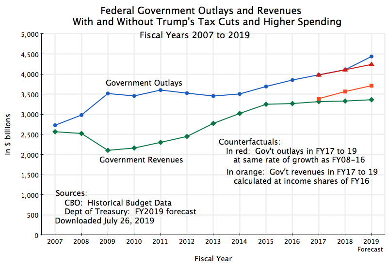
The chart at the top of this post shows what has happened. The deficit is the difference between what the government spends (shown as the line in blue) and the revenues it receives (the line in green). The deficit grew markedly following the financial and economic collapse in the last year of the Bush administration. A combination of higher government spending and lower taxes (lower both because the economy was depressed but also from legislated tax cuts) were then necessary to stabilize the economy. As the economy recovered the fiscal deficit then narrowed. But it is now widening again, and as noted above, is expected to top $1 trillion dollars in FY2019 (which ends on September 30).
More precisely, the US Treasury publishes monthly a detailed report on what the federal government received in revenues and what was spent in outlays for that month and for up to that point in the fiscal year. See here for the June report, and here for previous monthly reports. It includes a forecast of what will be received and spent for the fiscal year as a whole, and hence what the deficit will be, based on the budget report released each spring, usually in March. For FY2019, the forecast was of a deficit of $1.092 trillion. But these are forecasts, and comparing the forecasts made to the actuals realized over the last three fiscal years (FY2016 to18), government outlays were on average overestimated by 2.0% and government revenues by 2.2%. These are similar, and scaling the forecasts of government outlays and government revenues down by these ratios, the deficit would end up at $1.075 trillion. I used these scaled figures in the chart above.
The widening in the deficit in recent years is evident. The interesting question is why. For this one needs counterfactuals, of what the figures would have been if some alternative decisions had been made.
For government revenues (taxes of various kinds), the curve in orange show what they would have been had taxes remained at the same shares of the relevant income (depending on the tax) as they were in FY2016. Specifically, individual income taxes were kept at a constant share of personal income (as defined and estimated in the National Income and Product Accounts, or NIPA accounts, assembled by the Bureau of Economic Analysis, or BEA, of the US Department of Commerce); corporate profit taxes were kept at a constant share of corporate profits (as estimated in the NIPA accounts); payroll taxes (primarily Social Security taxes) were kept at a constant share of compensation of employees (again from the NIPA accounts); and all other taxes were kept at a constant share of GDP. The NIPA accounts (often referred to as the GDP accounts) are available through the second quarter of CY2019, and hence are not yet available for the final quarter of FY2019 (which ends September 30, and hence includes the third quarter of CY2019). For this, I extrapolated the final quarter’s figures based on what growth had been over the preceding four quarters.
Note also that the base year here (FY2016) already shows a flattening in tax revenues. If I had used the tax shares of FY2015 as a base for the comparison, the tax losses in the years since then would have been even greater. Various factors account for the flattening of tax revenues in FY2016, including (according to an analysis by the Congressional Budget Office) passage by Congress of Public Law 114-113 in December 2015, that allowed for a more rapid acceleration of depreciation allowances for investment by businesses. This had the effect of reducing corporate profit taxes substantially in FY2016.
Had taxes remained at the shares of the relevant income as they were in FY2016, tax revenues would have grown, following the path of the orange curve. Instead, they were flat in nominal dollar amount (the green curve), indicating they were falling in real terms as well as a share of income. The largest loss in revenues stemmed from the major tax cut pushed through Congress in December 2017, which took effect on January 1, 2018. Hence it applied over three of the four quarters in FY2018, and for all of FY2019.
An increase in government spending is also now leading, in FY2019, to a widening of the deficit. Again, one needs to define a counterfactual for the comparison. For this I assumed that government spending during Trump’s term in office so far would have grown at the same rate as it had during Obama’s eight years in office (the rate of increase from FY2008 to 16). That rate of increase during Obama’s two terms was 3.2% a year (in nominal terms), and was substantially less than during Bush’s two terms (which was a 6.6% rate of growth per year).
The rate of growth in government spending in the first two years of Trump’s term (FY2017 and 2018) then almost exactly matched the rate of growth under Obama. But this has now changed sharply in FY19, with government spending expected to jump by 8.0% in just one year.
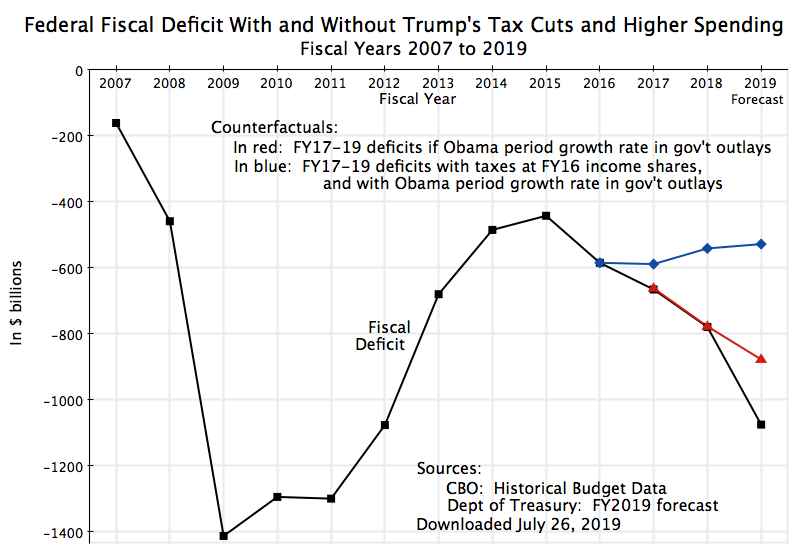
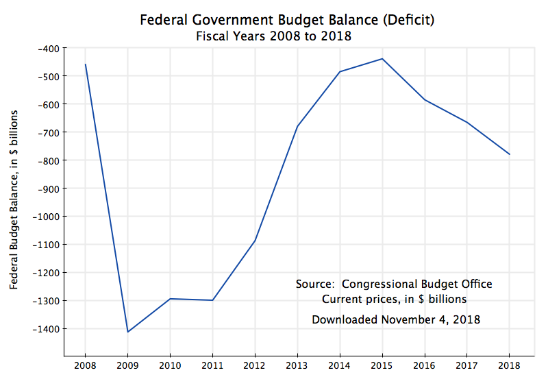
The fiscal deficit is then the difference, as noted above, between the two curves for spending and revenues. Its change over time may be clearer in a chart of just the deficit itself:

The curve in black shows what the deficit has been, and what is expected for FY2019. The deficit narrowed to $442 billion in FY2015, and then started to widen. Primarily due to flat tax revenues in FY2016 (spending was following the path it had been following before, after several years of suppression), the deficit grew in FY2016. And it then continued to grow until at least through FY2019. The curve in red shows what the deficit would have been had government spending continued to grow under Trump at the pace it had under Obama. This would have made essentially no difference in FY2017 and FY2018, but would have reduced the deficit in FY2019 from the expected $1,075 billion to $877 billion instead. Not a small deficit by any means, but not as high.
But more important has been the contribution to the higher deficit from tax cuts. The combined effect is shown in the curve in blue in the chart. The deficit would have stabilized and in fact reduced by a bit. For FY2019, the deficit would have been $528 billion, or a reasonable 2.5% of GDP. Instead, at an expected $1,075 billion, it will be over twice as high. And it is a consequence of Trump’s policies.
B. Have the Tax Cuts Led to Higher Growth?
The Trump administration claimed that the tax cuts (and specifically the major cuts passed in December 2017) would lead to such a more rapid pace of GDP growth that they would “pay for themselves”. This clearly has not happened – tax revenues have fallen in real terms (they were flat in nominal terms). But a less extreme argument was that the tax cuts, and in particular the extremely sharp cut in corporate profit taxes, would lead to a spurt of new corporate investment in equipment, which would raise productivity and hence GDP. See, for example, the analysis issued by the White House Council of Economic Advisors in October 2017.
But this has not happened either. Growth in private investment in equipment has in fact declined since the first quarter of 2018 (when the law went into effect):

The curve in blue shows the quarter to quarter changes (at an annual rate), while the curve in red smooths this out by showing the change over the same quarter of a year earlier. There is a good deal of volatility in the quarter to quarter figures, while the year on year changes show perhaps some trends that last perhaps two years or so, but with no evidence that the tax cut led to a spurt in such investment. The growth has in fact slowed.
Such investment is in fact driven largely by more fundamental factors, not by taxes. There was a sharp fall in 2008 as a result of the broad economic and financial collapse at the end of the Bush administration, it then bounced back in 2009/10, and has fluctuated since driven by various industry factors. For example, oil prices as well as agricultural prices both fell sharply in 2015, and the NIPA accounts indicate that equipment investment in just these two sectors reduced private investment in equipment by more than 2% points from what the total would have been in 2015. This continued into 2016, with a reduction of a further 1.3% points. What matters are the fundamentals. Taxes are secondary, at best.
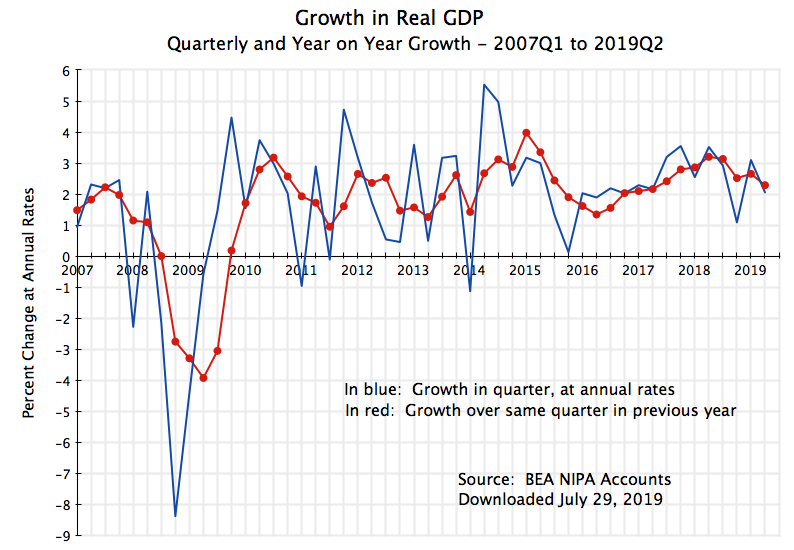
What about GDP itself?:
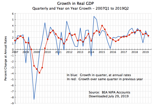
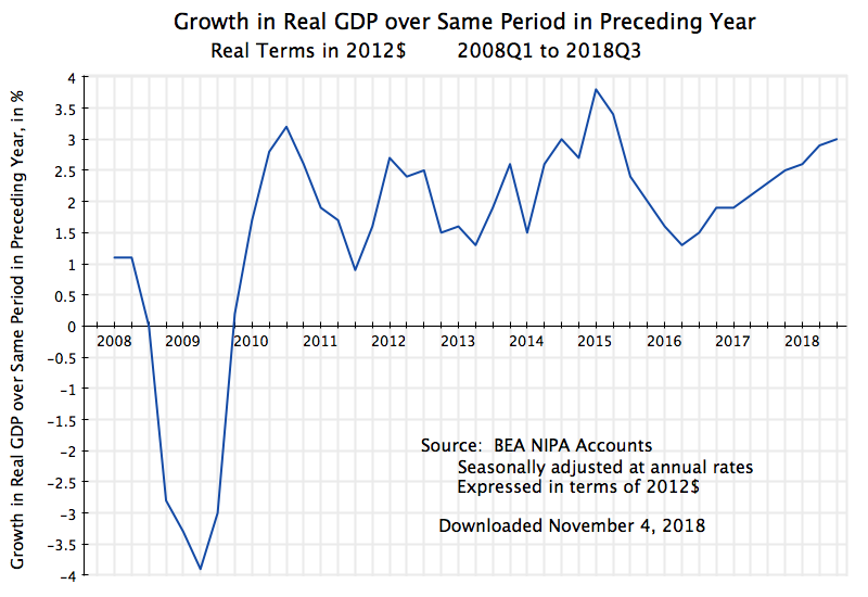
Here again there is quarter to quarter volatility, but no evidence that the tax cuts have spurred GDP growth. Over the past three years, real GDP growth on a quarter to quarter basis peaked in the fourth quarter of 2017, before the tax cuts went into effect, and has declined modestly since then. And that peak in the fourth quarter of 2017 was not anything special: GDP grew at a substantially faster pace in the second and third quarters of 2014, and the year on year rate in early 2015 was higher than anything reached in 2017-19. Rather, what we see in real GDP growth since late 2009 is significant quarter to quarter volatility, but around an average pace of about 2.3% a year. There is no evidence that the late 2017 tax cut has raised this.
The argument that tax cuts will spur private investment, and hence productivity and hence GDP, is a supply-side argument. There is no evidence in the numbers to support this. But there may also be a demand-side argument, which is basically Keynesian. The argument would be that tax cuts lead to higher (after-tax) incomes, and that these higher incomes led to higher consumption expenditures by households. There might be some basis to this, to the extent that a portion of the tax cuts went to low and middle-income households who will spend more upon receiving it. But since the tax cut law passed in December 2017 went primarily to the rich, whose consumption is not constrained by their current income flows (they save the excess), the impact of the tax cuts on household consumption would be weak. It still, however, might be something.
But this still did not lead to a more rapid pace of GDP growth, as we saw above. Why? One needs to recognize that GDP is a measure of production in the domestic economy (GDP is Gross Domestic Product), and not of demand. GDP is commonly measured by adding up the components of demand, with any increase or decrease in the stock of inventories then added (or subtracted, if negative) to tell us what production must have been. But this is being done because the data is better (and more quickly available) for the components of GDP demand. One must not forget that GDP is still an estimate of production, and not of total domestic demand.
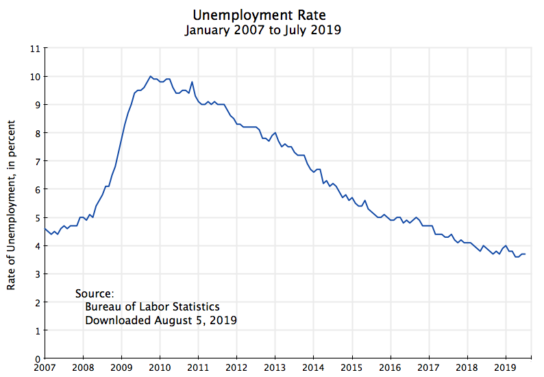
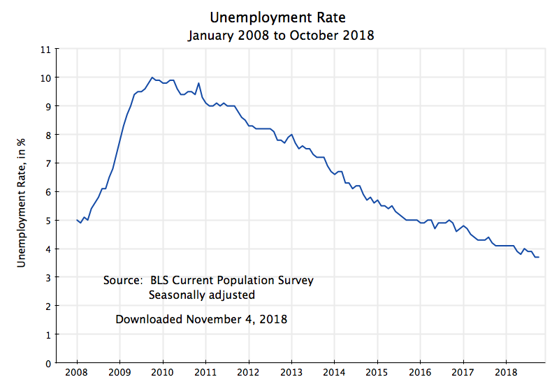
And what the economy can produce when at full employment is constrained by whatever capacity was at that point in time. The rate of unemployment has fallen steadily since hitting its peak in 2009 during the downturn:
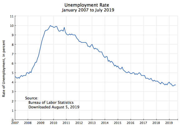 Aside from the “squiggles” in these monthly figures (the data are obtained from household surveys, and will be noisy), unemployment fell at a remarkably steady pace since 2009. One can also not discern any sharp change in that pace before and after January 2017, when Trump took office. But the rate of unemployment is now leveling off, as it must, since there will always be some degree of frictional unemployment when an economy is at “full employment”.
With the economy at full employment, growth will now be constrained by the pace of growth of the labor force (about 0.5% a year) plus the growth in productivity of the average labor force member (which analysts, such as at the Congressional Budget Office, put at about 1.5% a year in the long term, and a bit less over the next decade). That is, growth in GDP capacity will be 2% a year, or less, on average.
In such situations, Keynesian demand expansion will not raise the growth in GDP beyond that 2% rate. There will of course be quarter to quarter fluctuations (GDP growth estimates are volatile), but on average over time, one should not expect growth in excess of this.
But growth can be less. In a downturn, such as that suffered in 2008/09, GDP growth can drop well below capacity. Unemployment soars, and Keynesian demand stimulus is needed to stabilize the economy and return it to a growth path. Tax cuts (when focused on low and middle income households) can be stimulative. But especially stimulative in such circumstances is direct government spending, as such spending leads directly to people being hired and put to work.
Thus the expansion in government spending in 2008/09 (see the chart at the top of this post) was exactly what was needed in those circumstances. The mistake then was to hold government spending flat in nominal terms (and hence falling in real terms) between 2009 and 2014, even though unemployment, while falling, was still relatively high. That cut-back in government spending was unprecedented in a period of recovery from a downturn (over at least the past half-century in the US). And an earlier post on this blog estimated that had government spending been allowed to increase at the same pace as it had under Reagan following the 1982 downturn, the US economy would have fully recovered by 2012.
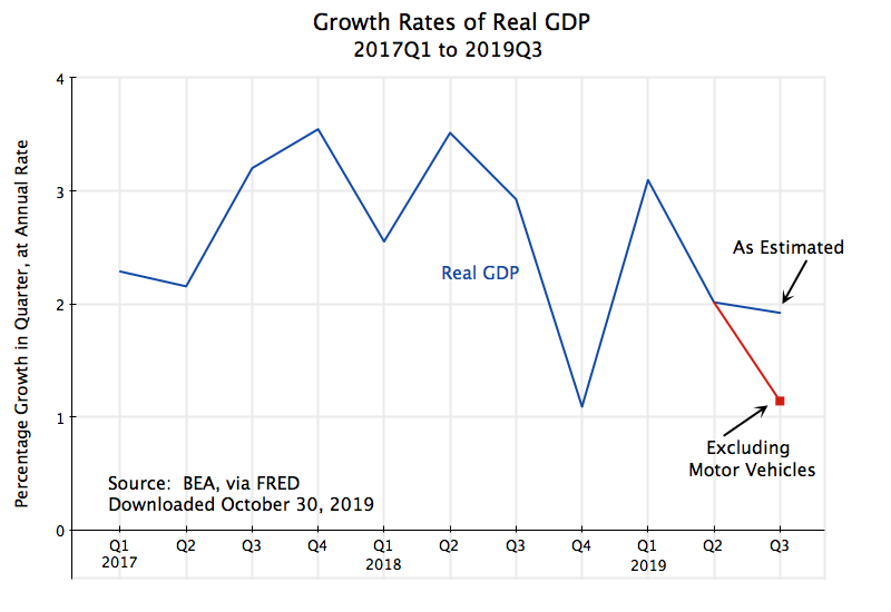
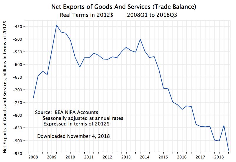
But the economy is now at full employment. In these circumstances, extra demand stimulus will not increase production (as production is limited by capacity), but will rather spill over into a drawdown in inventories (in the short term, but there is only so much in inventories that one can draw down) or an increase in the trade deficit (more imports to satisfy the domestic demand, or exports diverted to meet the domestic demand). One saw this in the initial estimates for the GDP figures for the second quarter of 2019. GDP is estimated to have grown at a 2.1% rate. But the domestic final demand components grew at a pace that, by themselves, would have accounted for a 3.6% point increase in GDP. The difference was accounted for by a drawdown in inventories (accounting for 0.7% points of GDP) and an increase in the trade deficit (accounting for a further reduction of 0.8% points of GDP). But these are just one quarter of figures, they are volatile, and it remains to be seen whether this will continue.
It is conceivable that domestic demand might fall back to grow in line with capacity. But this then brings up what should be considered the second arm of Trump’s Keynesian stimulus program. While tax cuts led to growing deficits in FY2017 and 18, we are now seeing in FY2019, in addition to the tax cuts, an extraordinary growth in government spending. Based on US Treasury forecasts for FY2019 (as adjusted above), federal government spending this fiscal year is expected to grow by 8.0%. This will add to domestic demand growth. And there has not been such growth in government spending during a time of full employment since George H. W. Bush was president.
C. The Impact of the Bipartisan Budget Act of 2019
Just before leaving for its summer recess, the House and the Senate in late July both passed an important bill setting the budget parameters for fiscal years 2020 and 2021. Trump signed it into law on August 2. It was needed as, under the budget sequester process forced on Obama in 2011, there would have otherwise been sharp cutbacks in the discretionary budgets for what government is allowed to spend (other than for programs such as Social Security or Medicare, where spending follows the terms of the programs as established, or for what is spent on interest on the public debt). The sequesters would have set sharp cuts in government spending in fiscal years 2020 and 2021, and if allowed, such sudden cuts could have pushed the US economy into a recession.
The impact is clear on a chart:
The figures are derived from the Congressional Budget Office analysis of the impact on government spending from the lifting of the caps. Without the change in the spending caps, discretionary spending would have been sharply reduced. At the new caps, spending will increase at a similar pace as it had before.
Note the sharp contrast with the cut-backs in discretionary budget outlays from FY2011 to FY2015. Unemployment was high then, and the economy struggled to recover from the 2008/09 downturn while confronting these contractionary headwinds. But the economy is now at full employment, and the extra stimulus on demand from such spending will not, in itself and in the near term, lead to an increase in capacity, and hence not lead to a faster rate of growth than what we have seen in recent years.
But I should hasten to add that lifting the spending caps was not a mistake. Government spending has been kept too limited for too long – there are urgent public needs (just look at the condition of our roads). And a sharp and sudden cut in spending could have pushed the economy into a recession, as noted above.
More fundamentally, keeping up a “high pressure” economy is not necessarily a mistake. One will of course need to monitor what is happening to inventories and the trade deficit, but the pressure on the labor market from a low unemployment rate has been bringing into the labor force workers who had previously been marginalized out of it. And while there is little evidence as yet that it has spurred higher wages, continued pressure to secure workers should at some point lead to this. What one does not want would be to reach the point where this leads to higher inflation. But there is no evidence that we are near that now. Indeed, the Fed decided on July 31 to reduce interest rates (for the first time since 2008, in part out of concern that inflation has been too low.
D. Summary, Implications, and Conclusion
Trump campaigned on the promise that he would bring down the government deficit – indeed bring it down to zero. The opposite has happened. The deficit has grown sharply, and is expected to reach over $1 trillion this fiscal year, or over 5% of GDP. This is unprecedented in the US in a time of full employment, other than during World War II.
The increase in the deficit is primarily due to the tax cuts he championed, supplemented (in FY2019) by a sharp rise in government spending. Without such tax cuts, and with government spending growth the same as it had been under Obama, the deficit in FY2019 would have been $530 billion. It is instead forecast to be double that (a forecast $1.075 trillion).
The tax cuts were justified by the administration by arguing that they would spur investment and hence growth. That has not happened. Growth in private investment in equipment has slowed since the major tax cuts of December 2017 were passed. So has the pace of GDP growth.
This should not be surprising. Taxes have at best a marginal effect on investment decisions. The decision to invest is driven primarily by more fundamental considerations, including whether the extra capacity is needed given demand for the products, by the technologies available, and so on.
But tax cuts (to the extent they go to low and middle income households), and even more so direct government spending, can spur demand in the economy. At times of less than full employment, this can lead to a higher GDP in standard Keynesian fashion. But when the economy is at full employment, the constraint is not aggregate demand but rather production capacity. And that is set by the available labor force and how much each worker can produce (their productivity). The economy can then grow only as fast as the labor force and productivity grow, and most estimates put that at about 2% or less per year in the US right now.
The spur to demand can, however, act to keep the economy from falling back into a recession. With the chaos being created in the markets by the trade wars Trump has launched, this is not a small consideration. Indeed, the Fed, in announcing its July 31 cut in interest rates, indicated that in addition to inflation tracking below its target rate of 2%, concerns regarding “global developments” (interpreted as especially trade issues) was a factor in making the cut.
There are also advantages to keeping high pressure on the labor markets, as it draws in labor that was previously marginalized, and should at some point lead to higher wages. As long as inflation remains modest (and as noted, it is currently below what the Fed considers desirable), all this sounds like a good situation. The fiscal policies are therefore providing support to help ensure the economy does not fall back into recession despite the chaos of the trade wars and other concerns, while keeping positive pressure in the labor markets. Trump should certainly thank Nancy Pelosi for the increases in the government spending caps under the recently approved budget agreement, as this will provide significant, and possibly critical, support to the economy in the period leading up to the 2020 election.
So what is there not to like?
The high fiscal deficit at a time of full employment is not to like. As noted above, a fiscal deficit of more than 5% of GDP during a time of full employment is unprecedented (other than during World War II). Unemployment was similarly low in the final few years of the Clinton presidency, but the economy then had fiscal surpluses (reaching 2.3% of GDP in FY2000) as well as a public debt that was falling in dollar amount (and even more so as a share of GDP).
The problem with a fiscal deficit of 5% of GDP with the economy at full employment is that when the economy next goes into a recession (and there eventually always has been a recession), the fiscal deficit will rise (and will need to rise) from this already high base. The fiscal deficit rose by close to 9 percentage points of GDP between FY2007 and FY2009. A similar economic downturn starting from a base where the deficit is already 5% of GDP would thus raise the fiscal deficit to 14% of GDP. And that would certainly lead conservatives to argue, as they did in 2009, that the nation cannot respond to the economic downturn with the increase in government spending that would be required to stabilize and then bring down unemployment.
Is a recession imminent? No one really knows, but the current economic expansion, that began five months after Obama took office, is now the longest on record in the US – 121 months as of July. It has just beaten the 120 month expansion during the 1990s, mostly when Clinton was in office. Of more concern to many analysts is that long-term interest rates (such as on 10-year US Treasury bonds) are now lower than short-term interest rates on otherwise similar US Treasury obligations. This is termed an “inverted yield curve”, as the yield curve (a plot of interest rates against the term of the bond) will normally be upward sloping. Longer-term loans normally have to pay a higher interest rate than shorter ones. But right now, 10-year US Treasury bonds are being sold in the market at a lower interest rate than the interest rate demanded on short-term obligations. This only makes sense if those in the market expect a downturn (forcing a reduction in interest rates) at some point in the next few years.
The concern is that in every single one of the seven economic recessions since the mid-1960s, the yield curve became inverted prior to that downturn. While this was typically two or three years before the downturn (and in the case leading up to the 1970 recession, about four years before), in no case was there an inverted yield curve without a subsequent downturn within that time frame. Some argue that “this time is different”, and perhaps it will be. But an inverted yield curve has been 100% accurate so far in predicting an imminent recession.
The extremely high fiscal deficit under Trump at a time of full employment is therefore leaving the US economy vulnerable when the next recession occurs. And a growing public debt (it will reach $16.8 trillion, or 79% of GDP, by September 30 of this year, in terms of debt held by the public) cannot keep growing forever.
What then to do? A sharp cut in government spending might well bring on the downturn that we are seeking to avoid. Plus government spending is critically needed in a range of areas. But raising taxes, and specifically raising taxes on the well-off who benefited disproportionately in the series of tax cuts by Reagan, Bush II, and then Trump, would have the effect of raising revenue without causing a contractionary impulse. The well-off are not constrained in what they spend on consumption by their incomes – they consume what they wish and save the residual.
The impact on the deficit and hence on the debt could also be significant. While now a bit dated, an analysis on this blog from September 2013 (using Congressional Budget Office figures) found that simply reversing in full the Bush tax cuts of 2001 and 2003 would lead the public debt to GDP ratio to fall and fall sharply (by about half in 25 years). The Trump tax cuts of December 2017 have now made things worse, but a good first step would be to reverse these.
It was the Bush and now Trump tax cuts that have put the fiscal accounts on an unsustainable trajectory. As was noted above, the fiscal accounts were in surplus at the end of the Clinton administration. But we now have a large and unprecedented deficit even when the economy is at full employment. In a situation like this, one would think it should be clear to acknowledge the mistake, and revert to what had worked well before.
Managing the fiscal accounts in a responsible way is certainly possible. But they have been terribly mismanaged by this administration.

 A. How Fast is GDP Growing?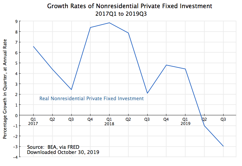







You must be logged in to post a comment.